Engee documentation
Notebook

Linear discriminant analysis (LDA)

This case study will examine the application of Linear Discriminant Analysis (LDA) to the Fisher's Iris dataset.A comparison with the Principal Component Analysis (PCA) method will also be made.

Linear discriminant analysis (LDA) is a statistical analysis technique that finds a linear combination of features to separate observations into two classes.

In [ ]:
Pkg.add(["MultivariateStats", "RDatasets"])
   Resolving package versions...
  No Changes to `~/.project/Project.toml`
  No Changes to `~/.project/Manifest.toml`

Suppose that the samples of positive and negative classes have mean values:

$\mu_p$ (for the positive class),

$\mu_n$ (for the negative class), and covariance matrices $C_p$ and $C_n$.

According to Fisher's criterion for the linear discriminant, the optimal projection direction is given by the formula: $$w = \alpha \cdot (C_p + C_n)^{-1} (\mu_p - \mu_n),$$ Where $\alpha$ is an arbitrary non-negative coefficient.

Installation and connection of necessary libraries:

In [ ]:
using MultivariateStats, RDatasets

Loading data from the Iris Fischer dataset:

In [ ]:
iris = dataset("datasets", "iris")
Out[0]:
150×5 DataFrame
125 rows omitted
RowSepalLengthSepalWidthPetalLengthPetalWidthSpecies
Float64Float64Float64Float64Cat…
15.13.51.40.2setosa
24.93.01.40.2setosa
34.73.21.30.2setosa
44.63.11.50.2setosa
55.03.61.40.2setosa
65.43.91.70.4setosa
74.63.41.40.3setosa
85.03.41.50.2setosa
94.42.91.40.2setosa
104.93.11.50.1setosa
115.43.71.50.2setosa
124.83.41.60.2setosa
134.83.01.40.1setosa
1396.03.04.81.8virginica
1406.93.15.42.1virginica
1416.73.15.62.4virginica
1426.93.15.12.3virginica
1435.82.75.11.9virginica
1446.83.25.92.3virginica
1456.73.35.72.5virginica
1466.73.05.22.3virginica
1476.32.55.01.9virginica
1486.53.05.22.0virginica
1496.23.45.42.3virginica
1505.93.05.11.8virginica

Extracting from the dataset the matrix of observation objects with features - X and the vector of classes of these objects - X_labels:

In [ ]:
X = Matrix(iris[1:2:end,1:4])'
X_labels = Vector(iris[1:2:end,5])
Out[0]:
75-element Vector{CategoricalArrays.CategoricalValue{String, UInt8}}:
 "setosa"
 "setosa"
 "setosa"
 "setosa"
 "setosa"
 "setosa"
 "setosa"
 "setosa"
 "setosa"
 "setosa"
 "setosa"
 "setosa"
 "setosa"
 ⋮
 "virginica"
 "virginica"
 "virginica"
 "virginica"
 "virginica"
 "virginica"
 "virginica"
 "virginica"
 "virginica"
 "virginica"
 "virginica"
 "virginica"

Let's compare linear discriminant analysis with PCA method (principal component analysis).

Training the PCA model:

In [ ]:
pca = fit(PCA, X; maxoutdim=2)
Out[0]:
PCA(indim = 4, outdim = 2, principalratio = 0.9741445733283195)

Pattern matrix (unstandardized loadings):
────────────────────────
         PC1         PC2
────────────────────────
1   0.70954    0.344711
2  -0.227592   0.29865
3   1.77976   -0.0797511
4   0.764206  -0.0453779
────────────────────────

Importance of components:
──────────────────────────────────────────────
                                PC1        PC2
──────────────────────────────────────────────
SS Loadings (Eigenvalues)  4.3068    0.216437
Variance explained         0.927532  0.0466128
Cumulative variance        0.927532  0.974145
Proportion explained       0.95215   0.04785
Cumulative proportion      0.95215   1.0
──────────────────────────────────────────────

Applying PCA to data:

In [ ]:
Ypca = predict(pca, X)
Out[0]:
2×75 Matrix{Float64}:
 2.71359    2.90321   2.75875   …  -2.39001   -1.51972   -1.87717
 0.238246  -0.233575  0.228345      0.333917  -0.297498   0.0985705

Training the LDA model:

In [ ]:
lda = fit(MulticlassLDA, X, X_labels; outdim=2);

Applying LDA to data:

In [ ]:
Ylda = predict(lda, X)
Out[0]:
2×75 Matrix{Float64}:
 -0.758539  -0.685016  -0.773267  …   0.976876   0.790049   0.84761
 -0.766144  -0.703192  -0.79546      -1.0143    -0.682331  -1.01696

Visualising the results:

In [ ]:
using Plots
p = plot(layout=(1,2), size=(800,300))

for s in ["setosa", "versicolor", "virginica"]

    points = Ypca[:,X_labels.==s]
    scatter!(p[1], points[1,:],points[2,:], label=s)
    points = Ylda[:,X_labels.==s]
    scatter!(p[2], points[1,:],points[2,:], label=false, legend=:bottomleft)

end
plot!(p[1], title="PCA")
plot!(p[2], title="LDA")
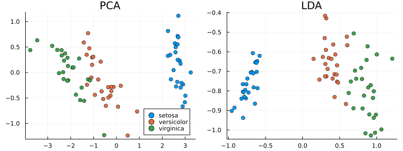
Out[0]:

Conclusions:

PCA and LDA are dimensionality reduction methods with different goals: PCA maximises the global variance of the data and is suitable for visualisation without considering class labels, whereas LDA optimises class separation using label information, making it effective for classification tasks. In the Fisher's Iris example, LDA provided a clear separation of classes in the projection, while PCA maintained the overall structure of the data but with overlapping classes. The choice of method depends on the task: PCA for exploring the data, LDA for improving classification in the presence of labelled classes.