Determining the distribution parameters for a partial sample
In this example, we will divide the sample into two parts and approximate each half with a separate probability density function using the least squares method to find the parameters of each function.
Creating a selection
Our sample will be a model of the Brownian process in the interval [-20, 20]. The particle transition occurs with equal probability to the left and to the right, the path length is determined by an exponential distribution with a given unit average.
We will get a set of implementations of this process by launching 100,000 trajectories from the center of the area.
Pkg.add(["Distributions", "Statistics", "Random",
         "StatsBase", "Measures", "HypothesisTests", "LsqFit"])
a = -20
b = 20
λ = 1

using Random
Random.seed!(2)

Ntraj = 100_000  # Number of calculated trajectories
Nc = []          # Set of trajectory lengths
NtrajList = []   # List of coordinates of the particle trajectory

for i in 1:Ntraj
    x = 0
    k = 0
    if length(NtrajList) < 200 push!( NtrajList, [] ); end
    while a < x < b
        r1,r2 = rand(2)
        dx = -log(r2) / λ
        if( r1 < 0.5 ) x -= dx; else x += dx; end;
        k += 1;
        # Let's save the first 200 trajectories in memory
        if length(NtrajList) < 200 push!( NtrajList[end], x ); end
    end
    Nc = push!( Nc, k )
end

Nc = Float64.( Nc );
We had to translate the vector Nc in type Float64, without which we would often receive warnings that the vector may contain data of the type Nothing or Missing even if they are not actually there.
Let's print the first couple hundred trajectories.
gr()

plot()
for traj in NtrajList
    plot!( 1:length(traj), traj, c=1 )
end

using Measures
plot!( legend=:false, size=(1000,400), xlabel="Simulation Steps", ylabel="Particle position", left_margin=10mm, bottom_margin=10mm )
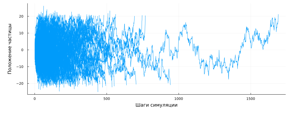
We can see that some particles have been in the controlled space for a very long time (up to 800 cycles or more), but mostly they left it during the first hundred steps from the start of the simulation.
Let's find the statistical parameters of this sample:
using Statistics
Nave = mean( Nc ); # The average value
Nd = std( Nc );    # Variance

histogram( Nc, xlims=(0,1000), normalize=true, label="Data" )
vline!( [Nave], lw=4, lc=2, label = "Average" )
vline!( [Nave+Nd], lw=3, lc=3, label=:none )
vline!( [Nave-Nd], lw=3, lc=3, label=:none )
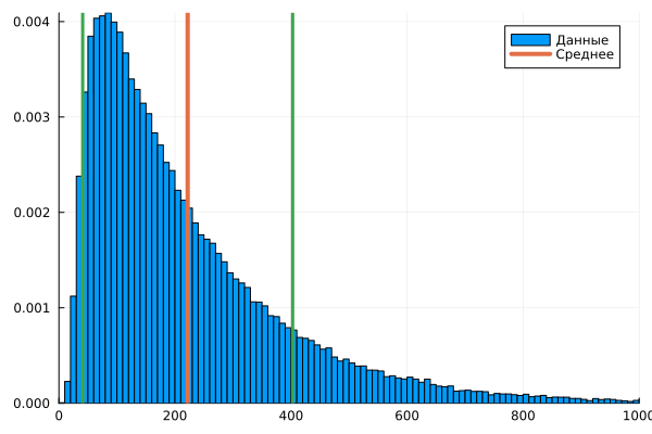
To examine this sample, the arithmetic mean is not enough. We need to guess which function is responsible for the distribution of the results of the observed process. To begin with, let's assume that we have a lognormal distribution in front of us.
using Distributions

dist0 = fit( LogNormal, Nc )
x1 = 10:1000

histogram( Nc, xlims=(0,1000), normalize=true, label="Data" )
plot!( x1, pdf.( dist0, x1 ), lw=4, lc=2, label="Lognormal distribution" )
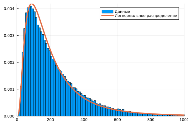
The right tail of the histogram is noticeably different in appearance from the curve of the found lognormal distribution.
Let's divide the data into two samples
Let's try to study two samples separately from each other. To do this, we divide the sample into two halves (before and after the maximum) and find the parameters of the two distribution functions. First of all, where is the maximum of the distribution?
xx = range( 10, 1000, step=8 )        # Histogram intervals
xc = xx[1:end-1] .+ (xx[2]-xx[1])/2   # Interval centers

# dist_h = fit( Histogram, Nc, xx ).weights; # The maximum of the histogram does not give the best estimate due to outliers,
dist_h = pdf.( dist0, x1 )                  # therefore, let's take the maximum of the lognormal function

m,i = findmax( dist_h )
Nc_mid = x1[i]
Let's separate the two subsamples:
Nc1 = Nc[ Nc .<= Nc_mid ];
Nc2 = Nc[ Nc .> Nc_mid ];
We approximate these two samples independently, one after the other. Let's build histograms based on them. Pay attention to the argument bins – if you do not specify it, the system will select a different interval size for each sample, and since we have different sample sizes, the density graph will be abnormal relative to the interval size.
histogram( Nc1 )
histogram!( Nc2, size=(600,150) )
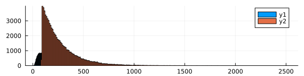
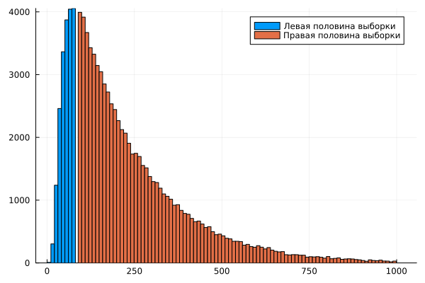
histogram( Nc1, bins=1:10:Nc_mid, label="The left half of the sample" )
histogram!( Nc2, bins=Nc_mid+1:10:1000, label="The right half of the sample" )
Now we have the weights of each interval obtained after plotting the histograms.
using StatsBase

# Interval boundaries for histograms
x1 = 10:Nc_mid
x2 = Nc_mid+1:1000

# Interval centers
c1 = x1[1:end-1] .+ (x1[2]-x1[1])/2
c2 = x2[1:end-1] .+ (x2[2]-x2[1])/2

# Histogram values (the third parameter is the interval boundaries)
w1 = fit( Histogram, Nc1, x1 ).weights;
w2 = fit( Histogram, Nc2, x2 ).weights;

# Normalized histograms (it is important to normalize using the entire length of Nc, rather than the length of individual tails)
w1n = w1 ./ length(Nc);
w2n = w2 ./ length(Nc);

plot( c1, w1n, label="The left half of the sample" )
plot!( c2, w2n, label="The right half of the sample" )
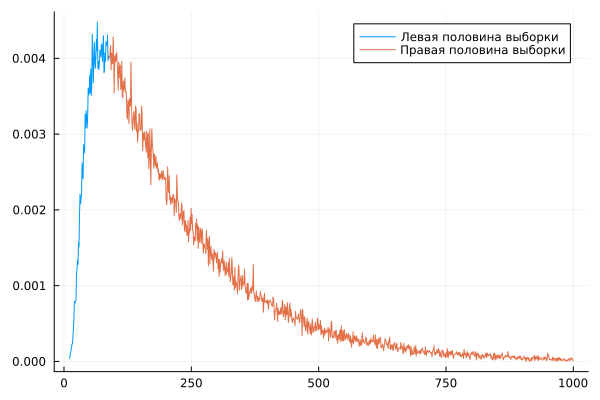
But each of them represents only a part of the data for constructing a histogram. Based on these data, it is impossible to fully find the distribution parameters, since we have a limited sample.
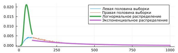
plot( c1, w1n, label="The left half of the sample" )
plot!( c2, w2n, label="The right half of the sample", size=(600,180) )

dist1 = fit( LogNormal, Nc1 )
dist2 = fit( Exponential, Nc2 )

plot!( c1, pdf.( dist1, c1 ), lw=4, label="Lognormal distribution" )
plot!( c2, pdf.( dist2, c2 ), lw=4, label="Exponential distribution" )
But on the other hand, we can find the distribution parameters if we set it as a function that must pass through the presented points.
Parameters of the left selection
Let's imagine that the left side of the distribution follows a lognormal law. This distribution has the following probability density formula:
This formula has two parameters – and , which we will have to form the elements of the vector p (p[1] and p[2]).
We will find the parameters of this curve with the condition that it should pass through the available points as closely as possible.
# Let's write the function by selecting function parameters (rather than distributions)
using LsqFit

# These functions must be written for vector arguments, so @. at the beginning (so that all operations are .*, .+, etc.)
@. lognormDist( x, p ) = (1 / (x * p[2] * sqrt(2π) )) * exp(-(log(x) - p[1])^2 / (2p[2]^2));

p0 = [1.0, 1.0];
af1 = curve_fit( lognormDist, c1, w1n, p0 );

af1.param
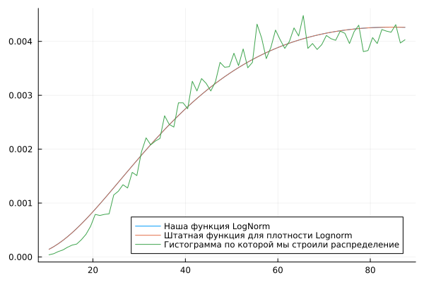
We have selected distribution parameters that give us a probability density very similar to that given by the built-in function. LogNormal.
plot( c1, lognormDist(c1, af1.param), label="Our LogNorm function", legend=:topleft )
plot!( c1, pdf.(LogNormal(af1.param[1], af1.param[2]), c1), label="Standard function for Lognorm density" )
plot!( c1, w1n, label="The histogram that we used to build the distribution", legend=:bottomright )
Parameters of the right selection
Let's try to fit the points of the "right" half of the sample into an exponential probability density function.:
Sometimes this distribution is constructed using a one-parameter function, but in our case, the results are better if .
@. expDist( x, p ) = p[1] * exp( -p[2]*x );

p0 = [ 0.1, 0.1]; # Everything depends very much on the initial parameter. At values above 0.5, the model does not converge.
af2 = curve_fit( expDist, c2, w2n, p0 );

af2.param
Since we use an iterative method to approximate the sample using a given function, we need to specify the initial approximation of the solution. p_0, the choice of which often determines whether our algorithm will converge or not.
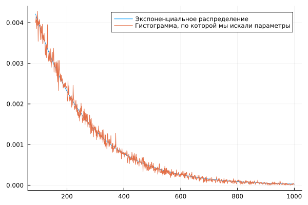
plot( c2, expDist(c2, af2.param), label="Exponential distribution" )
plot!( c2, w2n, label="The histogram that we used to search for parameters" )
Both parts are compatible
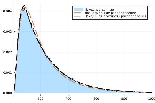
If we put both functions on the same graph, we will get a pretty good match with the original histogram, as we can verify with the help of the package HypothesisTests.
stephist( Nc, xlims=(10,1000), bins = 10:5:1000, normalize=true, label="Initial data", fill=true, fillalpha=0.3, color=:black, fillcolor=1 )
plot!( [c1; c2], pdf.( dist0, [c1; c2] ), lw=3, lc=2, ls=:dash, label="Lognormal distribution" )
plot!( [c1; c2], [lognormDist(c1, af1.param); expDist(c2, af2.param)], lw=3, lc=:black, ls=:dash, label="The found distribution density" )
Let's evaluate the quality of this solution.
We have actually written a piecewise linear function into the sample. Now let's evaluate the residual error, both visually and using the Student's criterion.
using HypothesisTests

yy1 = pdf.( dist0, [c1; c2] )
yy2 = [ lognormDist(c1, af1.param); expDist(c2, af2.param) ]
yy3 = [w1n; w2n]

plot(
    plot( yy1 .- yy3, size=(600,250), lc=2,
        label="Lognorm (pvalue = $(round(pvalue(OneSampleTTest(yy1 .- yy3)),digits=3)))" ),
    plot( yy2 .- yy3, size=(600,250), lc=1,
        label="Lognorm + Exponential (pvalue=$(round(pvalue(OneSampleTTest(yy2 .- yy3)),digits=3)))" ),
    layout=(2,1)
)
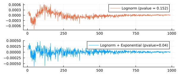
The second error graph looks more uniform.
-the value shows that we have taken into account more systematic effects, and that the error between the sample and the function we have compiled is closer to a normally distributed random variable than the error between the sample and the distribution function. LogNorm.
Conclusion
We solved an application problem for which we needed to fit several functions into the samples. As a result, we have constructed a complex distribution function to describe the results of a physical experiment.