Interpolation and extrapolation
Interpolation is a technique that allows you to supplement a data set with missing values calculated at points located between the available points in the sample. Interpolation can be used to fill in gaps in data, smooth out outliers, predict process behavior, and so on. To estimate values outside the experimental definition area, extrapolation methods are used.
Unlike different types of regression or polynomial approximation, for interpolation, it is desirable that the source data be located on a regular grid. In other words, the arguments to the function must be specified using the data type. Range. Function , which performs output data interpolation y set on the grid x, we will call the interpolating function or interpolant.
Multidimensional interpolation on a grid
With enough data points, you can get a forecast at any intermediate point, including on a regular grid or on a random sample of points.
Pkg.add(["Interpolations"])
using Interpolations, Plots, Random
Random.seed!(12);
gr( fmt=:png, size=(500,400) );
Let's assume that our empirical data forms a 4-by-4 matrix:
xs = range( 1, 10, length=4 );
ys = range( 1, 10, length=4 );
zs = rand( length(xs), length(ys) );
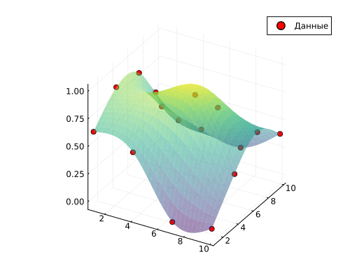
By creating the interpolant we need (for example, through a cubic spline), we can calculate its value at any point within the input data range.:
itp = cubic_spline_interpolation( (xs,ys), zs );
itp( 2, 2 )
This model will allow us to calculate the output values at any point within the argument space, bounded by the perimeter defined by the grid on which empirical data is defined.
Let's plot the interpolation result on a new grid with a small step size between the points.
scatter( repeat(xs, inner=length(ys)),
         repeat(ys, outer=length(xs)),
         vec(reshape( zs, (1,:))), markercolor=:red, label="Data" )

xs_new = range(1, 10, length=30)
ys_new = range(1, 10, length=30)
surface!( xs_new, ys_new, [itp(x,y) for x in xs_new, y in ys_new],
          colorbar = false, alpha = 0.5, c=:viridis )
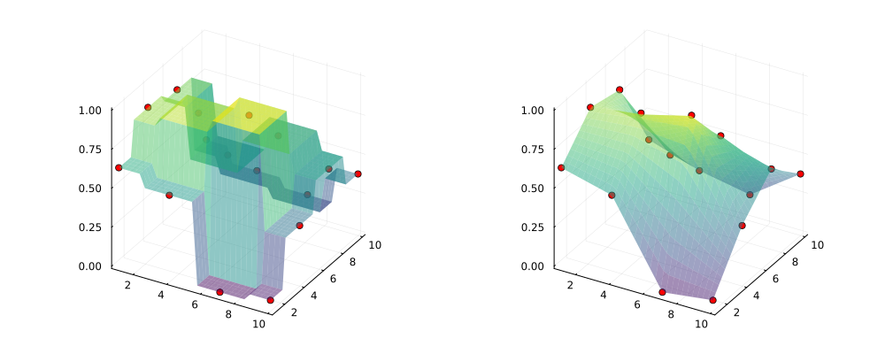
We used the command for linear interpolation: cubic_spline_interpolation and when it was created, two vectors of arguments and a grid of values were passed to it as input. This function allows you to get forecasts for individual pairs of arguments or create an entire forecast matrix.
Piecewise linear interpolation can be performed in the same way (linear_interpolation) or "nearest neighbor method" interpolation (constant_interpolation). Exactly the same actions can be implemented using the commands ConstantInterpolation, LinearInterpolation and CubicSplineInterpolation. According to the documentation, they were left in the library for convenience.
itp0 = constant_interpolation( (xs,ys), zs ); # The constant
itp1 = linear_interpolation( (xs,ys), zs ); # Linear interpolation

plot(
    (scatter( repeat(xs, inner=length(ys)), repeat(ys, outer=length(xs)), vec(reshape( zs, (1,:))), markercolor=:red );
     surface!( xs_new, ys_new, itp0(xs_new, ys_new), colorbar = false, alpha = 0.5, c=:viridis, legend=:none )
     ),
    (scatter( repeat(xs, inner=length(ys)), repeat(ys, outer=length(xs)), vec(reshape( zs, (1,:))), markercolor=:red );
     surface!( xs_new, ys_new, itp1(xs_new, ys_new), colorbar = false, alpha = 0.5, c=:viridis, legend=:none )
     ),
    size=(1000,400)
    )
The type of interpolation function is determined by the degree of the polynomial defining the spline: Constant, Linear, Quadratic, or Cubic. So far, we have used the convenient, simplified syntax of these commands. But there is also a more complex syntax.:
# Calculating the interpolation by a quadratic spline,
# specifying the boundary condition – Reflect
# and interpreting the points on the periphery as centroids (OnCell)
# we also additionally scale the resulting interpolant, which, with this syntax, initially has a single range.
sitp4 = scale( interpolate(zs, BSpline(Quadratic(Reflect(OnCell())))), (xs, ys,))

# Linear interpolation on one axis, stepwise interpolation on the other axis
# the Gridded argument means that the points on the perimeter are interpreted as OnGrid()
itp5 = interpolate( (xs, ys), zs, (Gridded(Linear()),Gridded(Constant())) )

plot(
    (scatter( repeat(xs, inner=length(ys)), repeat(ys, outer=length(xs)), vec(reshape( zs, (1,:))), markercolor=:red );
     surface!( xs_new, ys_new, sitp4(xs_new, ys_new), colorbar = false, alpha = 0.5, c=:viridis, legend=:none )
    ),

    (scatter( repeat(xs, inner=length(ys)), repeat(ys, outer=length(xs)), vec(reshape( zs, (1,:))), markercolor=:red );
     surface!( xs_new, ys_new, itp5(xs_new, ys_new), colorbar = false, alpha = 0.5, c=:viridis, legend=:none )
    ),
    size=(1000,400)
)
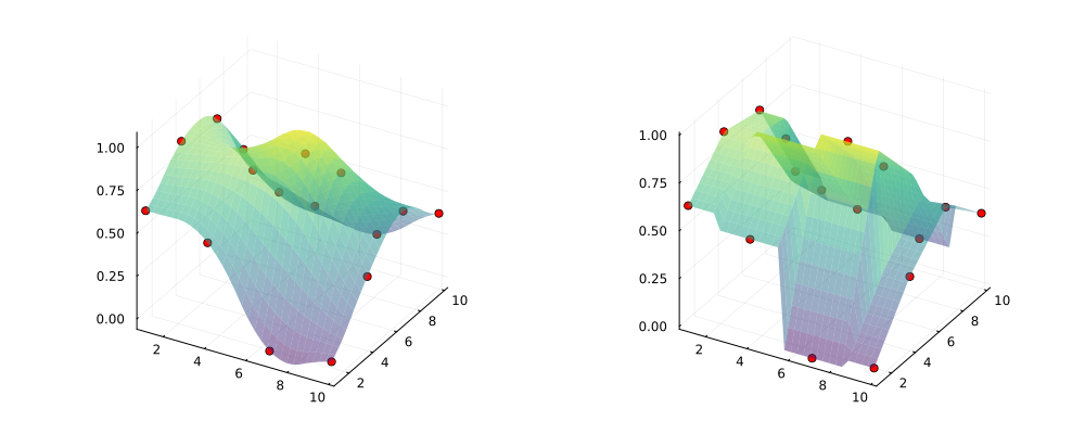
Not all combinations of conditions can produce results. For example, quadratic and cubic interpolation require specifying boundary conditions from the list. Flat, Line (the same as Natural), Free, Periodic or Reflect. The points on the perimeter of the grid can be interpreted by the interpolation algorithm as boundary points (OnGrid()) or as being located halfway between the preceding row and the fictitious next row of points (OnCell()).
The interpolation of data set on an irregular grid can be performed using a piecewise linear spline and using constants.
Information about additional parameters and interpolation modes can be found [in the documentation] (https://engee.com/helpcenter/stable/julia/Interpolations/interpolations.html ).
Extrapolation
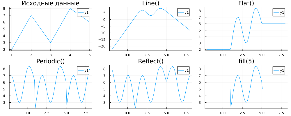
If it is necessary to predict data outside the range of available experimental data, we need to add another hypothesis to the interpolation parameters – how, in our opinion, the function behaves outside the available data, and here we have options. Throw (issue an error), Flat, Line, Periodic and Reflect, or you can pass a constant as an argument, the value of which will be substituted during interpolation.
We will demonstrate different extrapolation methods using the example of a one-dimensional signal.
x = 1:5;
y = [2,7,3,8,6];
Setting different boundary conditions (boundary conditions) using the argument extrapolation_bc.
new_x = range(-2, 8, length=100)

plot(
    plot(x, y, title="Initial data"),
    plot(new_x, cubic_spline_interpolation(x, y, extrapolation_bc=Line())(new_x), title="Line()"),
    plot(new_x, cubic_spline_interpolation(x, y, extrapolation_bc=Flat())(new_x), title="Flat()"),
    plot(new_x, cubic_spline_interpolation(x, y, extrapolation_bc=Periodic())(new_x), title="Periodic()"),
    plot(new_x, cubic_spline_interpolation(x, y, extrapolation_bc=Reflect())(new_x), title="Reflect()"),
    plot(new_x, cubic_spline_interpolation(x, y, extrapolation_bc=5)(new_x), title="fill(5)"),
    size=(1000,400), layout=(2,3)
)
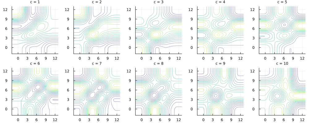
Of course, these same methods allow for the interpolation and extrapolation of higher dimensional data. For example, let's place 64 data points in 3-dimensional space and construct a smooth function based on them.
a = range( 1, 10, length=4 );
b = range( 1, 10, length=4 );
c = range( 1, 10, length=4 );
d = rand( length(a), length(b), length(c) );

# 3D interpolation (easy to write in one line)
itp = extrapolate(
          scale(
              interpolate( d, BSpline(
                                  Quadratic(
                                      Reflect(OnCell())
                                  )
                              )
                ), (a,b,c,)
      ), Flat() )

# Setting a new grid
new_a = new_b = -2:0.1:13; new_c = 1:10;

vPlots = [ contour( new_a, new_b, itp(new_a, new_b, ic), colorbar = false, alpha = 0.5, c=:viridis, legend=:none, title="c = $ic", titlefont = font(8)) for ic in new_c ]
plot!( vPlots..., layout=(2,:), size=(1000,400) )
Conclusion
We have reviewed several data interpolation methods that can be used with data of any dimension. The interpolation methods we have studied allow us to work with the initial data set on the grids. For non-ordered data, it is better to use classical machine learning methods or advanced visualization methods (for example, through Delaunay triangulation).
There are several dozen more packages in the Julia ecosystem for data interpolation in other problem settings, a list of them is given on [this page] (https://juliamath.github.io/Interpolations.jl/stable/other_packages /).