Regression using a multilayer neural network¶

In this work, we will need to train a neural network to predict the output of a continuous function from two parameters and place it on the Engee canvas as another block. For example, as a surrogate model to replace some complex subsystem.

Data description¶

Our data is generated by a process of the form $y = f(x_1, x_2)$:

Pkg.add(["JLD2", "Flux"])

Nx1, Nx2 = 30, 40
x1 = Float32.( range( -3, 3, length=Nx1 ) )
x2 = Float32.( range( -3, 3, length=Nx2 ) )
Xs = [ repeat( x1, outer=Nx2)  repeat( x2, inner=Nx1) ];
# Первый пример выходных данных
Ys = @. 3*(1-Xs[:,1])^2*exp(-(Xs[:,1]^2) - (Xs[:,2]+1)^2) - 10*(Xs[:,1]/5 - Xs[:,1]^3 - Xs[:,2]^5)*exp(-Xs[:,1]^2-Xs[:,2]^2) - 1/3*exp(-(Xs[:,1]+1) ^ 2 - Xs[:,2]^2);
# Второй пример выходных данных
#Ys = @. 1*(1-Xs[:,1])^2*exp(-(Xs[:,1]^2) - (Xs[:,2]+1)^2) - 15*(Xs[:,1]/5 - Xs[:,1]^3 - Xs[:,2]^6)*exp(-Xs[:,1]^2-Xs[:,2]^2) - 1/3*exp(-(Xs[:,1]+1) ^ 2 - Xs[:,2]^2);

Xs - matrix of size 1200x2 (there are 1200 examples in the sample, each characterised by two features: x1 and x2)

Ys - matrix of size 1200х1 (forecast column)

Learning process¶

Let's set the parameters for the learning procedure and run a fairly simple version of the loop.

# @markdown ## Настройка параметров нейросети
# @markdown *(двойной клик позволяет скрыть код)*
# @markdown
Параметры_по_умолчанию = false #@param {type: "boolean"}
if Параметры_по_умолчанию
    Коэффициент_скорости_обучения = 0.01
    Количество_циклов_обучения = 2000
else
    Количество_циклов_обучения = 2001 # @param {type:"slider", min:1, max:2001, step:10}
    Коэффициент_скорости_обучения = 0.08 # @param {type:"slider", min:0.001, max:0.5, step:0.001}
end

epochs = Количество_циклов_обучения;
learning_rate = Коэффициент_скорости_обучения;

Let us create a neural network with two inputs, two intermediate states (of size 20 and 5) and one output. It is important that the neural network output has a linear activation function.

using Flux
model = Chain( Dense( 2 => 20, relu ),      # Структура модели, которую мы будем обучать
               Dense( 20 => 5, relu ),
               Dense( 5 => 1 ) )
data = [ (Xs', Ys') ]                       # Зададим структуру данных
loss( ỹ, y ) = Flux.mse( ỹ, y )             # и функцию потерь, в которую они будут передаваться процедурой обучения
loss_history = []                           # Будем сохранять историю обучения
opt_state = Flux.setup( Adam( learning_rate ), model ); # Алгоритм оптимизации
for i in 1:epochs
    Flux.train!( model, data, opt_state) do m, x, y
        loss( m(x), y ) # Функция потерь - ошибка на каждом элементе датасета
    end
    push!( loss_history, loss( model(Xs'), Ys' ) ) # Запомним значение функции потерь
end
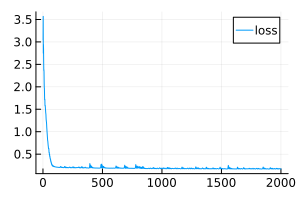
plot( loss_history, size=(300,200), label="loss" ) # Выведем хронику обучения

Transfer the neural network to the Engee canvas¶

The variable model stores the newly trained neural network.

We have recreated its structure using elements on the canvas:

☝️ Our model needs the variable model, from where it gets the parameters. If this variable does not exist, the model will try to find the file model.jld2 in the home directory. If this file is not found, the model will create an empty neural network with random parameters

Fully connected layers are built from the most common blocks Product and Add, multiplying inputs by a matrix and adding a vector of offsets.

Activation functions, for clarity, are not hidden inside layers, but outside.

Let's run this model on a set of several hundred random points.

if "neural_regression_multilayer" ∉ getfield.(engee.get_all_models(), :name)
    engee.load( "$(@__DIR__)/neural_regression_multilayer.engee");
end
model_data = engee.run( "neural_regression_multilayer" );

The model returns us a matrix of matrices. You can fix this with canvas blocks, or you can implement your own variant of the function flatten:

model_x1 = model_data["X1"].value;
model_x2 = model_data["X2"].value;
model_y = vec( hcat( model_data["Y"].value... ));

Conclusion results¶

gr()

plot(
    surface( Xs[:,1], Xs[:,2], vec(Ys), c=:viridis, cbar=:false, title="Обучающая выборка", titlefont=font(10)),
    wireframe( x1, x2, vec(model( Xs' )), title="Прогноз от нейросети (через скрипт)", titlefont=font(10) ),
    scatter( model_x1, model_x2, model_y, ms=2.5, msw=.5, leg=false, zcolor=model_y,
        xlimits=(-3,3), ylimits=(-3,3), title="Прогноз от модели на холсте", titlefont=font(10) ),
    layout=(1,3), size=(1000,400)
)

Save the model¶

Finally, let's save the trained neural network to a file if this file is missing.

if !isfile( "model.jld2" )
    using JLD2
    jldsave("model.jld2"; model)
end

Conclusion¶

We trained a multilayer neural network consisting of three fully connected layers. We then transferred all its coefficients to a canvas for use in a convenient model-oriented context (more convenient than working with neural networks through code).

It is easy to repeat this work with any tabular data and scale the neural network to fit the needs of the project. Saving the trained network to a file allows you to run the model along with other elements of the Engee diagram without having to re-train the neural network.

If desired, weights and offsets can be written to Constant blocks on the canvas to produce a neural network block independent of the presence of the model.jld2 file.