Identification of model parameters in Engee
Description of the example
Let's consider the implementation of the problem of parametric identification of a model based on data. We have to determine several time-invariant parameters of a certain model, the structure of which is known to us in advance.
In this example, we will analyze the signal generated by the dynamic model Engee. It is located in the folder start/examples/data_analysis/parametric_identification.
The model consists of two subsystems: one generates the analyzed signal, the other is a reference model (without noise).
In the subsystem ModelSystem using summation, five signals are combined:
- Constant component: number 5,
- time component: a line with a slope of 0.01,
- first harmonic: a sine wave with an amplitude of 1 and an angular frequency glad/with,
- less noticeable second harmonic: a sine wave with an amplitude of 0.6 and an angular frequency glad/with,
- White noise with zero offset and 0.3 variance.
.png)
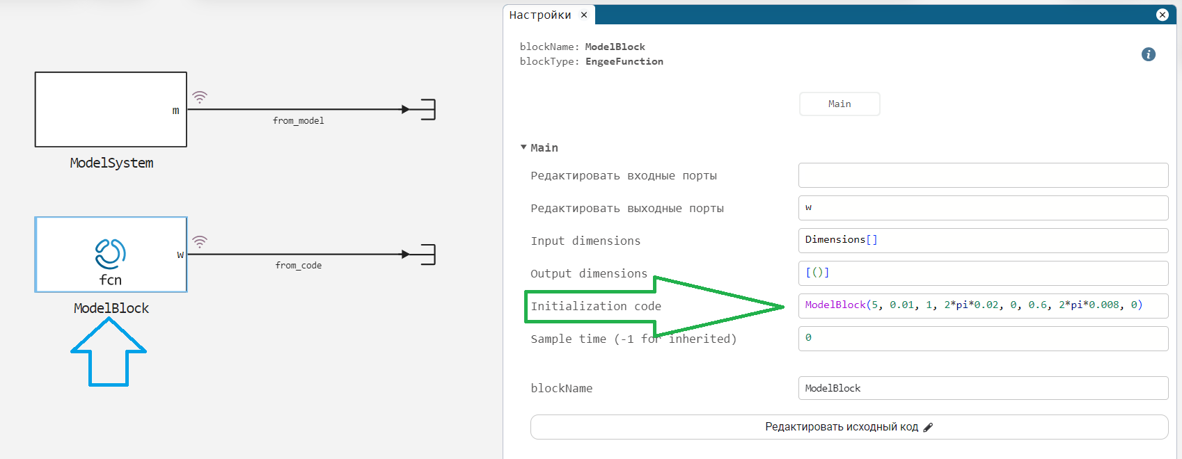
In the subsystem ModelBlock we will be able to substitute the identified parameters. So far, reference parameters have been set in it and it generates a reference signal. It describes the model in the form of a code:
function (c::ModelBlock)(t::Real)
    T0 = 5
    T1 = 0.01
    A1, f1, phi1 = 1, 0.02, 0
    A2, f2, phi2 = 0.6, 0.008, 0

    signal = T0 + T1 * t +
             A1 * sin( 2*pi * f1 * t + phi1 ) .+
             A2 * sin( 2*pi * f2 * t + phi2 );
    return signal
end
Let's save the reference values of the parameters:
Pkg.add(["CSV", "HypothesisTests"])
# "Ideal" parameters of the linear part of the signal (offset, slope)
T0m = 5;
T1m = 0.01;
# The "ideal" parameters of the first sinusoid (amplitude, frequency, phase)
A1m = 1;
f1m = 0.02;
phi1m = 0;
# The "ideal" parameters of the second sine wave (amplitude, frequency, phase)
A2m = 0.6;
f2m = 0.008;
phi2m = 0;
As a result of running the model, we get 500 seconds of signal. Here is a graph of the last 200 seconds:
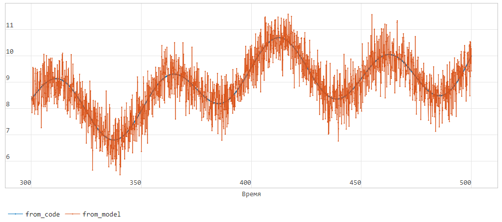
Block ModelBlock it is currently being initialized with exactly the same parameters as the dynamic model in the subsystem. ModelSystem, therefore , the graph from_code (dark blue) completely repeats the systematic part of the signal from_model (orange color).
What data does the model save?
Both signals are saved in the CSV table param_id_data.csv with the following columns:
time– time column,m– a column of data generated by the dynamic model (reference parameters and error),c– a column of data generated by the reference model (executed as code).
The procedure in this example is
We have to perform the following actions:
- Run a dynamic model to synthesize the model data
- select the parameters of all the links of the model in the correct order (we assume that the signal allows us to guess the topology of the model, or that we already know it)
- check that after subtracting the systematic components from the input signal, a normally distributed noise is obtained
- insert the parameters into the Engee Function block code and check how well the models match each other.
Synthesis of model data
To synthesize the data that we will analyze, run the following cell:
modelName = "param_identification_model"
# engee.close( modelName, force=true ) # To restart the model
model = modelName in [m.name for m in engee.get_all_models()] ? engee.open( modelName ) : engee.load( "$(@__DIR__)/$modelName.engee");

results = engee.run( modelName, verbose=false )
Loading libraries
Connect libraries for downloading data, working with tables, analyzing spectra, and libraries for polynomial regression.
using CSV, DataFrames, FFTW, Polynomials
Downloading and connecting a library to test hypotheses (we use normality testing):
# import Pkg; Pkg.add( "HypothesisTests", io=devnull );
using HypothesisTests
Upload the data
Next, we will only work with the signal generated from the dynamic model, but you can make sure that both methods are interchangeable, and if necessary, this example can fit into just one script.
We will visualize the model's signal. ModelSystem, which consists of a time vector and calculated values:
t = results["from_model"].time;
signal = results["from_model"].value;
We will also save the sampling frequency of the time signal (the inverse of the time distance between two adjacent measurements):
sample_rate = 1/(t[2] - t[1])
What will we identify
The reference model ModelBlock it is initialized with reference parameter values (the same as in the model ModelSystem).
.png)
The model is defined by 8 parameters:
- Linear trend parameters:
- the amplitude, frequency, and phase of the first sine wave:
- amplitude, frequency, and phase of the second sine wave:
We will not be interested in noise parameters, although they are easy to identify with functions. mean and var.
We identify the linear component
First of all, we identify and remove a linear trend from the signal.
trend = Polynomials.fit( t, signal, 1 ) # Last argument: the degree of the polynomial
Saving the parameters of the polynomial in separate variables
T0, T1 = trend[0], trend[1]
Let's display the found trend on the graph and show what our data looks like minus this trend.:
plot(
    plot( t, [signal trend.(t)], label=["Data" "The trend"] ),
    plot(t, signal - trend.(t), lc=:darkblue, label="Trendless"),
    layout=(2,1)
)
Great, the signal looks like a combination of sine waves and noise.
We identify the first sinusoid
To determine the parameters of the sinusoids included in the signal, we will plot the signal spectrum using the FFTW library.
The sampling of which will be proportional to the number of points in the original signal. That is, if we leave the original sampling, we can get a low accuracy of the spectrum. To get rid of the high-frequency region, we will reduce the number of points in the original signal by lowering the sampling frequency of the original signal. To do this, we set a variable downsample_factor. A value of 40 means that we will take every 40th point from the original signal.
downsample_factor = 40;

# Next, we will work with a low-sampling signal (signal_downsampled)
idx_downsample = 1:downsample_factor:length(t)
t_downsampled = t[idx_downsample]

# Sampling of the signal from which we subtracted the linear trend
signal_downsampled = (signal - trend.(t))[idx_downsample];
Since we are only interested in the positive part of the spectrum, we use the function rfft (we also won't have to do fftshift):
# Let's find the spectrum of the signal
F1 = rfft(signal_downsampled)

# Calculate the frequency vector of the found spectrum
freqs = rfftfreq(length(t_downsampled), sample_rate/downsample_factor)

# Let's output a graph
plot( freqs, abs.(F1) )
Let's find the maximum on this spectrum and determine which frequency this value corresponds to.
_,idx = findmax( abs.(F1) )
print( "The frequency of the most noticeable component: ", freqs[idx] )
When we have found the maximum point on the spectrum, we can identify the amplitude, frequency, and phase of the most prominent harmonic component. Now we need to do recombination – generate a harmonic signal from a complex number that describes its parameters.
# We find the parameters of the sine wave
A1 = 2 * abs( F1[idx] ) ./ length(t_downsampled )
# Multiplication by 2 occurs due to the fact that the signal power in the spectrum
# it is divided between two peaks: positive and negative

f1 = abs( freqs[idx] ) # The frequency of the sine wave
phi1 = angle( F1[idx] ) + pi/2 # The phase of the sine wave

print("A1 = ", A1, "\nf1 = ", f1, "\nphi1 = ", phi1)
Let's set the first sinusoid as a function of time and output a graph:
# A function that defines a sinusoid with the found parameters
sinusoid1(tt) = A1 * sin.( 2*pi*f1*tt .+ phi1 );

# We display graphs
plot(
    plot( t, [signal .- trend.(t), sinusoid1.(t)], label=["Data without a linear trend" "The first sinusoid"]  ),
    plot( t, signal .- trend.(t) .- sinusoid1(t), lc=:darkblue, label="Residual signal" ),
    layout=(2,1)
)
Okay, now the signal is a combination of a sine wave and noise.
Identify the second sinusoid
Let's repeat the same operations as for searching for the first sinusoid.:
# Downsampling signal (without trend and first sinusoid)
signal_downsampled2 = (signal .- trend.(t) .- sinusoid1(t))[idx_downsample]

# We find the spectrum of the signal after subtracting the first two components
F2 = rfft(signal_downsampled2)

# Calculate the frequency vector of the found spectrum
freqs = rfftfreq(length(t_downsampled), sample_rate/downsample_factor)

# Let's output a graph
plot( freqs, abs.(F2) )
Let's find the parameters of the second sinusoid
# We find the maximum on the spectrum
_,idx2 = findmax( abs.(F2) )

# We determine the parameters of the sine wave corresponding to this maximum
A2 = 2 * abs( F2[idx2] ) ./ length( t_downsampled ) # The amplitude
f2 = abs( freqs[idx2] ) # Frequency
phi2 = angle( F2[idx2] ) + pi/2 # Phase

print( "A2 = ", A2, "\nf2 = ", f2, "\nphi2 = ", phi2 )
Let's set the second sinusoid as a function of time and output a graph:
# A function that defines a sinusoid with the found parameters
sinusoid2(tt) = A2 * sin.( 2*pi*f2*tt .+ phi2 );

# We display graphs
plot(
    plot(t, [signal.-trend.(t).-sinusoid1.(t) sinusoid2.(t)],
        label = ["The signal minus two components" "The second sinusoid"]),
    plot(t, signal.-trend.(t).-sinusoid1(t).-sinusoid2(t), lc=:darkblue,
        label = "Residual signal", legend=:outertopright),
    layout=(2,1)
)
How do I find out if there are still significant systematic components in this signal? One way is to imagine that this signal is a realization of a random variable and check it for the normality of the distribution.
Residual signal analysis
Let's test the hypothesis about the normal distribution of the residual component of the signal using test Харке-Бера (JB test):
h = JarqueBeraTest( signal .- trend.(t) .- sinusoid1(t) .- sinusoid2(t) )
Pay attention to the result (outcome) of the test:
fail to reject h_0This means that there is no good reason to reject the hypothesis. With 95% confidence, we state that the observed signal is generated by a random process with a normal distributionreject h_0this means that the confidence that the observed signal originates from a normal distribution does not exceed 5%
Try to exclude some component from the formula - most likely, such a signal will not pass test Харке-Бера and you will get the result reject h_0.
Analysis of the results
The result obtained serves as the basis for completing the search for additional systematic components.
We will display the final report and the error in estimating the parameters.
df = DataFrame(
    ["T0"    T0    T0m    string(round(100*abs(T0 - T0m)/T0m, digits=2))*"%";
     "T1"    T1    T1m    string(round(100*abs(T1 - T1m)/T1m, digits=2))*"%";
     "A1"    A1    A1m    string(round(100*abs(A1 - A1m)/A1m, digits=2))*"%";
     "f1"    f1    f1m    string(round(100*abs(f1 - f1m)/f1m, digits=2))*"%";
     "phi1"  phi1  phi1m  string(round(abs(phi1 - phi1m),digits=2))*" glad";
     "A2"    A2    A2m    string(round(100*abs(A2 - A2m)/A2m, digits=2))*"%";
     "f2"    f2    f2m    string(round(100*abs(f2 - f2m)/f2m, digits=2))*"%";
     "phi2"  phi2  phi2m  string(round(abs(phi2 - phi2m),digits=2))*" glad"
    ],
    ["Parameter", "Identified", "Model value", "Error rate"]
 )
Let's create a function that calculates data from a model with identified parameters.:
function ModelBlock(t)
    global T0, T1, A1, f1, phi1, A2, f2, phi2;

    signal = T0 .+ T1 .* t .+
          A1 .* sin.( 2*pi .* f1 .* t + phi1 ) .+
          A2 .* sin.( 2*pi .* f2 .* t + phi2);

    return signal
end;
Let's compare the result of executing the identified model and the result of launching it. ModelBlock:
plot( results["from_model"].time,
          [results["from_model"].value, results["from_code"].value, ModelBlock.(t) ],
      label=["The original signal" "The reference model" "The identified model"],
      linecolor=[:lightblue :red :green])
In this example, we:
- implemented a fairly simple parametric identification procedure,
- the error of identification of all parameters has been determined,
- we made sure that the graph of the model with the identified parameters is quite similar to the graph of the reference model.