Approaches to the design of neural regulators
Webinar Разработка перспективных видов регуляторов для объектов управления в Engee it consisted of several examples:
This project contains the accompanying materials for the third part of the webinar, and you can study the rest in the community using the links above.
An example with a regular PID controller
This is the main model in which we will replace the regulator.
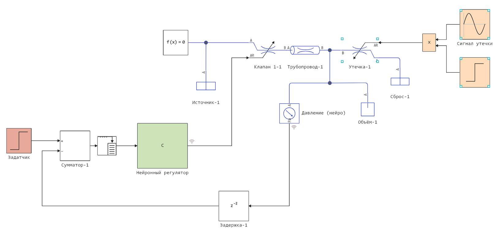
The liquid_pressure_regulator.engee model
Adaptive PID controller
First of all, we will set up an adaptive PID controller, the coefficients of which go through the following update procedure with each time step.:
    if abs(e) > c.thr
        c.Kp = max(0, c.Kp + clamp(c.α*e*c.pe, -c.ΔK, c.ΔK))
        c.Ki = max(0, c.Ki + clamp(c.α*e*c.pie, -c.ΔK, c.ΔK))
        c.Kd = max(0, c.Kd + clamp(c.α*e*c.pde, -c.ΔK, c.ΔK))
    end
First, we will not react to jumps in the control signal larger than a certain size. c.thr (parameter threshold). Secondly, the parameter α limits the rate of change of all parameters of the controller, while the step of change is modulo limited by the parameter ΔK.
.png)
The liquid_pressure_regulator_adaptive_pid.engee model
Neural regulator on Julia (RNN)
This controller contains the code of a recurrent neural network running on Julia without high-level libraries. His training takes place "online", during the operation of the system, so the quality of his work depends very much on the initial values of his weights. It may be necessary to apply a pre-training procedure, at least so that the neural network begins to produce a stable value when the pipeline state is stationary at the beginning of the calculation.
.png)
The liquid_pressure_regulator_neural_test.engee model
Creating a neural controller in C (FNN)
Let's launch the model and assemble the dataset
Pkg.add("CSV")
using DataFrames, CSV
engee.open("$(@__DIR__)/liquid_pressure_regulator.engee")
data = engee.run( "liquid_pressure_regulator" )
function simout_to_df( data )
    vec_names = [i for i in keys(data) if length(data[i].value) > 0];
    df = DataFrame( hcat([collect(data[v]).value for v in vec_names]...), vec_names );
    df.time = collect(data[vec_names[1]]).time;
    return df
end
df = simout_to_df( data );
CSV.write("Mode 1.csv", df);
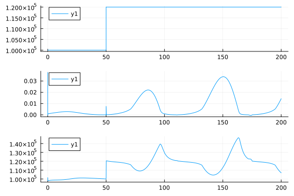
plot(
plot( df.time, df.set_point ), plot( df.time, df.control ), plot( df.time, df.pressure ), layout=(3,1)
)

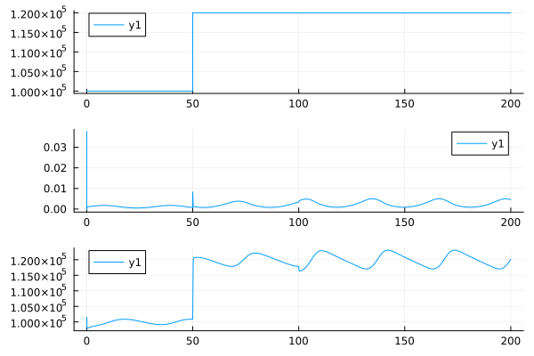
Let's change the parameters of the model and run it in a different scenario.
engee.set_param!( "liquid_pressure_regulator/Сигнал утечки", "Amplitude"=>"0.001" )
data = engee.run( "liquid_pressure_regulator" )
df = simout_to_df( data );
CSV.write("Mode 2.csv", df);
plot(
    plot( df.time, df.set_point ), plot( df.time, df.control ), plot( df.time, df.pressure ), layout=(3,1)
)
engee.set_param!( "liquid_pressure_regulator/Сигнал утечки", "Amplitude"=>"0.0005", "Frequency"=>"0.2" )
data = engee.run( "liquid_pressure_regulator" )
df = simout_to_df( data );
CSV.write("3.csv mode", df);
plot(
    plot( df.time, df.set_point ), plot( df.time, df.control ), plot( df.time, df.pressure ), layout=(3,1)
)
Putting all the model parameters back in place
engee.set_param!( "liquid_pressure_regulator/Сигнал утечки", "Amplitude"=>"0.0005" )
engee.set_param!( "liquid_pressure_regulator/Сигнал утечки", "Frequency"=>"0.1" )
Let's train a neural network to approximate several regulators
This code allows you to prepare data, sets the structure of a three-layer fully connected neural network, and trains it to find the relationship between the past 20 mismatch values and the next control signal value.
Pkg.add(["Flux", "BSON", "Glob", "MLUtils"])
using Flux, MLUtils
using CSV, DataFrames
using Statistics, Random
using BSON, Glob
# Initialize the random number generator for the sake of reproducibility of the experiment
Random.seed!(42)
# 1. Prepare the data
function load_and_preprocess_data_fnn()
# Download all CSV files from the current folder
files = glob("*.csv")
dfs = [CSV.read(file, DataFrame, types=Float32) for file in files]
# Combine data into one table
combined_df = vcat(dfs...)
# Let's extract the columns we need (time, error, control)
vtime = combined_df.time
error = combined_df.error
control = combined_df.control
# Data normalization (will greatly help with speeding up neural network learning)
error_mean, error_std = mean(error), std(error)
control_mean, control_std = mean(control), std(control)
error_norm = (error .- error_mean) ./ error_std
control_norm = (control .- control_mean) ./ control_std
# We divide it into small sequences to train the RNN
sequence_length = 20 # how many past steps do we take into account to predict the control signal
X = []
Y = []
for i in 1:(length(vtime)-sequence_length)
push!(X, error_norm[i:i+sequence_length-1])
push!(Y, control_norm[i+sequence_length])
end
# Formalize them as arrays
# X = reshape(hcat(X...), sequence_length, 1, :) # With butches
X = hcat(X...)'
Y = hcat(Y...)'
return (X, Y), (error_mean, error_std, control_mean, control_std)
end
# 2. We define the structure of the model
function create_fnn_controller(input_size=20, hidden_size=5, output_size=1)
return Chain(
Dense(input_size, hidden_size, relu),
Dense(hidden_size, hidden_size, relu),
Dense(hidden_size, output_size)
)
end
# 3. Learning with the new Flux API
function train_fnn_model(X, Y; epochs=100, batch_size=32)
# Data separation
split_idx = floor(Int, 0.8 * size(X, 1))
X_train, Y_train = X[1:split_idx, :], Y[1:split_idx, :]
X_val, Y_val = X[split_idx+1:end, :], Y[split_idx+1:end, :]
# Creating a model and optimizer
model = create_fnn_controller()
optimizer = Flux.setup(Adam(0.001), model)
# Loss function
loss(x, y) = Flux.mse(model(x), y)
# Preparing the DataLoader
train_loader = Flux.DataLoader((X_train', Y_train'), batchsize=batch_size, shuffle=true)
# The learning cycle
train_losses = []
val_losses = []
for epoch in 1:epochs
# Training
Flux.train!(model, train_loader, optimizer) do m, x, y
y_pred = m(x)
Flux.mse(y_pred, y)
end
# Error calculation
train_loss = loss(X_train', Y_train')
val_loss = loss(X_val', Y_val')
push!(train_losses, train_loss)
push!(val_losses, val_loss)
# Logging
if epochs % 10 == 0
@info "Epoch $epoch" train_loss val_loss
end
end
# Visualization of learning
plot(1:epochs, train_losses, label="Training Loss")
plot!(1:epochs, val_losses, label="Validation Loss")
xlabel!("Epoch")
ylabel!("Loss")
title!("Training Progress")
return model
end
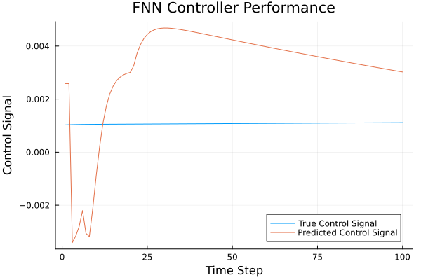
# 4. Evaluation of the model (unchanged)
function evaluate_fnn_model(model, X, Y, norm_params)
predictions = model(X')
# Denormalization
_, _, control_mean, control_std = norm_params
Y_true = Y .* control_std .+ control_mean
Y_pred = predictions' .* control_std .+ control_mean
# Calculation of metrics
rmse = sqrt(mean((Y_true - Y_pred).^2))
println("RMSE: ", rmse)
# Visualization
plot(Y_true[1:100], label="True Control Signal")
plot!(Y_pred[1:100], label="Predicted Control Signal")
xlabel!("Time Step")
ylabel!("Control Signal")
title!("FNN Controller Performance")
end
# Uploading data
(X, Y), norm_params = load_and_preprocess_data_fnn()

# Training
model = train_fnn_model(X, Y, epochs=100, batch_size=32)

# Saving the model
using BSON
BSON.@save "fnn_controller_v2.bson" model norm_params
# Evaluation
evaluate_fnn_model(model, X, Y, norm_params)
Let's generate the C code for a fully connected neural network.
Let's apply the library Symbolics to generate the code, we will make several improvements so that it can be called from the block. C Function.
Pkg.add("Symbolics")
using Symbolics
@variables X[1:20]
c_model_code = build_function( model( collect(X) ), collect(X); target=Symbolics.CTarget(), fname="neural_net", lhsname=:y, rhsnames=[:x] )
# Let's replace a few instructions in the code
c_fixed_model_code = replace( c_model_code,
                              "double" => "float",
                              "f0" => "f",
                              "  y[0]"=>"y" );

println( c_fixed_model_code[1:200] )
println("...")
# Let's leave only the third line of this code.
c_fixed_model_code = split(c_fixed_model_code, "\n")[3]

c_code_standalone = """
float ifelse(bool cond, float a, float b) { return cond ? a : b; }

$c_fixed_model_code""";

println( c_code_standalone[1:200] )
println("...")
Save the code to a file
open("$(@__DIR__)/neural_net_fc.c", "w") do f
    println( f, "$c_code_standalone" )
end
.png)
The liquid_pressure_regulator_neural_fc.engee model
Conclusion
Obviously, we have been training neural networks for too short a time using too small an example. There are many steps that should make it possible to improve the quality of such a controller - for example, to apply more signals to the input of a neural network, or simply assemble a larger dataset for better offline learning. We have shown how to approach the development of a neural regulator and how to test it in the Engee model environment.