Synthesis of antenna array radiation patterns using deep learning
The example demonstrates how to design and train a convolutional neural network that calculates the weights of antenna array elements to form the required pattern of the radiation pattern.
Introduction
The weights of the grid elements allow you to form a radiation pattern in such a way that it corresponds to a given one.
Deep learning methods have shown excellent results in computer vision and natural language processing in recent years. Despite the fact that neural network training takes time and is conducted offline, after training, the network is able to instantly produce results. This makes it possible to synthesize patterns in real time.
Importing libraries
!pip install -r /user/Demo_public/data_analysis/directional_pattern/requirements.txt
In this example, an exploratory data analysis will be performed, including an initial inspection of the set structure, studying the distributions of features and the target variable, identifying omissions, outliers and duplicates, as well as analyzing correlations between variables. At the next stage, regression models will be built and trained in order to predict the target variable and evaluate the quality of their work using appropriate metrics. Additionally, an analysis of the importance of the features will be performed, which will determine which of them make the greatest contribution to the predictions of the model and can be considered the most significant for the task under study.
import os, glob, time, datetime, copy
import numpy as np
import cvxpy as cp
import matplotlib.pyplot as plt

import torch
import torch.nn as nn
import torch.nn.functional as F
from torch.utils.data import Dataset, DataLoader, random_split
from torchvision import transforms, models
from PIL import Image
Define auxiliary functions
Visualization
DB_FLOOR = -80
def plot_pattern_cut(az_grid, el_grid, pat_db, el0=0.0, title=None):
    idx = int(np.argmin(np.abs(el_grid - el0)))
    plt.figure(figsize=(6,4.2))
    plt.plot(az_grid, pat_db[idx, :])
    plt.xlabel('Azimuth'); plt.ylabel('Relative level, dB')
    plt.title(title); plt.grid(True); plt.tight_layout(); plt.show()

def plot_pattern_2d(az_grid, el_grid, pat_db, db_floor=-60, title='Beam Pattern'):
    pat_db = np.clip(pat_db, db_floor, 0)
    AZ, EL = np.meshgrid(az_grid, el_grid)
    plt.figure(figsize=(6.6,5.2))
    cf = plt.contourf(AZ, EL, pat_db, levels=40)
    plt.contour(AZ, EL, pat_db, levels=np.arange(db_floor, 1, 5), colors='k', linewidths=0.4, alpha=0.4)
    plt.colorbar(cf, label='dB')
    plt.xlabel('Azimuth (deg)'); plt.ylabel('Elevation (deg)')
    plt.title(title); plt.tight_layout(); plt.show()

def plot_aperture(pos, r):
    y, z = pos[:,1], pos[:,2]
    plt.figure(figsize=(5,5))
    plt.scatter(y, z, s=80)
    circ = plt.Circle((0,0), r, fill=False, ls='--', lw=1.5)
    plt.gca().add_artist(circ)
    plt.gca().set_aspect('equal', 'box')
    plt.xlabel('y (m)'); plt.ylabel('z (m)')
    plt.grid(True, alpha=0.3)
    plt.tight_layout(); plt.show()
Synthesis of weights
def get_circular_planar_positions(r=3.0, delta=0.5, wavelength=1.0):
    ys = np.arange(-r, r + 1e-9, delta)
    zs = np.arange(-r, r + 1e-9, delta)
    Y, Z = np.meshgrid(ys, zs, indexing='xy')
    mask = (Y**2 + Z**2) <= r**2 + 1e-9
    y = Y[mask].ravel()
    z = Z[mask].ravel()
    x = np.zeros_like(y)
    pos = np.c_[x, y, z] / wavelength
    return pos.astype(float), pos.shape[0]

def dir_unit_vector(az_deg, el_deg):
    az = np.deg2rad(az_deg); el = np.deg2rad(el_deg)
    c = np.cos(el)
    return np.array([c*np.cos(az), c*np.sin(az), np.sin(el)])

def steering_vector(pos, az_deg, el_deg):
    u = dir_unit_vector(az_deg, el_deg)
    phase = 2*np.pi * (pos @ u)
    return np.exp(1j * phase)

def steering_matrix(pos, az_list, el_list):
    A = []
    for az, el in zip(az_list, el_list):
        A.append(steering_vector(pos, az, el).conj())
    return np.vstack(A) if A else np.zeros((0, pos.shape[0]), dtype=complex)

def array_response_fast(pos, w, az_grid, el_grid):
    az = np.deg2rad(np.asarray(az_grid))
    el = np.deg2rad(np.asarray(el_grid))
    ca, sa = np.cos(az), np.sin(az)
    ce, se = np.cos(el), np.sin(el)
    ux = np.outer(ce, ca)
    uy = np.outer(ce, sa)
    uz = np.outer(se, np.ones_like(az))
    phase = 2*np.pi * (pos[:,0,None,None]*ux + pos[:,1,None,None]*uy + pos[:,2,None,None]*uz)
    A = np.exp(1j*phase)
    val = np.tensordot(np.conj(A), w, axes=(0,0))
    pat = 20*np.log10(np.maximum(np.abs(val), 1e-12))
    pat -= np.max(pat)
    return pat

def make_side_region(az_span, el_span, step=0.5, exclude=set()):
    azs = np.arange(az_span[0], az_span[1] + 1e-9, step)
    els = np.arange(el_span[0], el_span[1] + 1e-9, step)
    return [(az, el) for az in azs for el in els if (az, el) not in exclude]

def db2lin_amp(db): return 10**(db/20.0)

def synthesize_mask_l2(pos, main_dir, null_dirs=None, null_db=None,
                       side_dirs=None, side_db=None):
    a_d = steering_vector(pos, *main_dir).conj()
    A_i = steering_matrix(pos, *(zip(*null_dirs)) if null_dirs else ([], []))
    A_s = steering_matrix(pos, *(zip(*side_dirs)) if side_dirs else ([], []))
    N = pos.shape[0]
    w = cp.Variable(N, complex=True)
    cons = [a_d @ w == 1]
    if A_i.size and null_db is not None:
        r_i = np.atleast_1d(null_db)
        r_i = np.full(A_i.shape[0], db2lin_amp(r_i[0])) if r_i.size==1 else db2lin_amp(r_i)
        cons += [cp.abs(A_i @ w) <= r_i]
    if A_s.size and side_db is not None:
        r_s = np.atleast_1d(side_db)
        r_s = np.full(A_s.shape[0], db2lin_amp(r_s[0])) if r_s.size==1 else db2lin_amp(r_s)
        cons += [cp.abs(A_s @ w) <= r_s]
    prob = cp.Problem(cp.Minimize(cp.norm(w, 2)), cons)
    prob.solve(verbose=False)
    if w.value is None: raise RuntimeError("Optimization didn't add up")
    return np.asarray(w.value).ravel()

def normalize_weights(w, ref_idx=0):
    w = w / (np.linalg.norm(w) + 1e-12)
    w *= np.exp(-1j*np.angle(w[ref_idx]))
    return w

def align_scale_phase(w_hat, w_true):

    alpha = (np.vdot(w_hat, w_true) / (np.vdot(w_hat, w_hat) + 1e-12))
    return alpha * w_hat


def db_to_uint8(pat_db, db_floor=DB_FLOOR):
    pat = np.clip(pat_db, db_floor, 0.0)
    img01 = (pat - db_floor) / (0.0 - db_floor)
    return (img01 * 255.0).astype(np.uint8)
Let's set the variables
LR              = 1e-4
WEIGHT_DECAY    = 1e-2
SEED            = 123
SAVE_DIR        = "./beam_ds_simple"
NUM_SAMPLES     = 1500
IMAGE_SIZE      = 224
DB_FLOOR        = -80.0
BATCH_SIZE      = 32
EPOCHS          = 20
MODEL_PATH      = "beamformer_resnet18.pth"

RADIUS  = 3.0
DELTA   = 0.5
LAMBDA  = 1.0
Grids
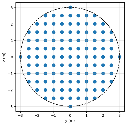
Consider a circular flat antenna array with a radius of 3 meters. The elements are arranged on a rectangular grid in 0.5 meter increments.
To generate coordinates, consider the function get_circular_planar_positions
r, delta, lamb = RADIUS, DELTA, LAMBDA
pos, N = get_circular_planar_positions(r, delta, lamb)
plot_aperture(pos, r=r)
Template synthesis using optimization
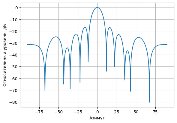
Suppose that you want to create a directional pattern in which the main lobe is oriented to the azimuth and the angle of the location is 0 °. The template must meet the following conditions::
- Maximize focus;
- Suppress interference at 30 dB below the main lobe;
- Ensure the level of the side lobes in the range from -20° to 20° in azimuth or elevation angle not higher than -17 dB relative to the main lobe.
main_dir = (0.0, 0.0)
interfs = [(12.0, 10.0), (13.0, 10.0)]
interfs_db = [-30.0, -30.0]
az_bands = [(-20, -10), (10, 20)]
el_bands = [(-20, -10), (10, 20)]

exclude = set(interfs)
side_pts = []
for az_span in az_bands:
    for el_span in el_bands:
        side_pts += make_side_region(az_span, el_span, step=0.5, exclude=exclude)
Synthesizing the lattice weights
w1 = synthesize_mask_l2(
    pos, main_dir,
    null_dirs=interfs, null_db=interfs_db,
    side_dirs=side_pts, side_db=-17.0
)
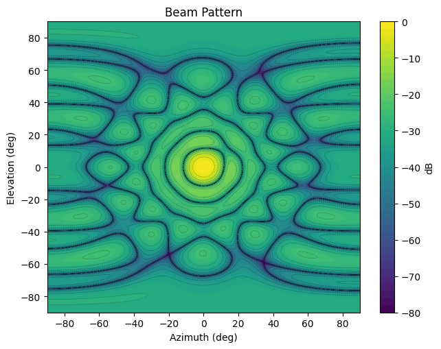
We get the lattice pattern
az_plot = np.arange(-90, 90.001, 0.25)
el_plot = np.arange(-90, 90.001, 0.25)

pat1 = array_response_fast(pos, w1, az_plot, el_plot)
plot_pattern_cut(az_plot, el_plot, pat1, el0=0.0)
plot_pattern_2d(az_plot, el_plot, pat1, db_floor=-80)
Next, you need to generate a dataset. To do this, we will use a separate function that iterates through the parameters on the basis of which the lattice is synthesized.
def generate_and_save(n=300, save_dir="./beam_ds", seed=42):

    rng = np.random.default_rng(seed)
    os.makedirs(save_dir, exist_ok=True)

    r, delta, lamb = 3.0, 0.5, 1.0
    pos, N = get_circular_planar_positions(r, delta, lamb)

    az_plot = np.arange(-90, 90.001, 0.25)
    el_plot = np.arange(-90, 90.001, 0.25)

    file_paths = []

    for i in range(n):
        main_dir = (rng.uniform(-5, 5), rng.uniform(-3, 3))

        K = int(rng.integers(1, 4))
        interfs = []
        for _ in range(K):
            interfs.append((
                rng.uniform(8, 25),
                rng.uniform(8, 15)
            ))
        interfs_db = list(rng.uniform(-35, -25, size=K))

        shift = rng.uniform(-3, 3)
        az_bands = [(-20+shift, -10+shift), (10+shift, 20+shift)]
        el_bands = [(-20, -10), (10, 20)]
        exclude = set((float(a), float(e)) for a, e in interfs)

        side_pts = []
        for az_span in az_bands:
            for el_span in el_bands:
                side_pts += make_side_region(az_span, el_span, step=0.5, exclude=exclude)

        side_db = -17.0

        w = synthesize_mask_l2(
            pos, main_dir,
            null_dirs=interfs, null_db=interfs_db,
            side_dirs=side_pts, side_db=side_db
        )
        pat_db = array_response_fast(pos, w, az_plot, el_plot)


        out_path = os.path.join(save_dir, f"sample_{i:05d}.npz")
        np.savez_compressed(
            out_path,

            pos=pos.astype(np.float32),
            weights=w.astype(np.complex64),
            pattern_db=pat_db.astype(np.float32),
            r=np.float32(r), delta=np.float32(delta), wavelength=np.float32(lamb),
            main_dir=np.array(main_dir, dtype=np.float32),
            interfs=np.array(interfs, dtype=np.float32),
            interfs_db=np.array(interfs_db, dtype=np.float32),
            side_db=np.float32(side_db),
            az_plot=az_plot.astype(np.float32),
            el_plot=el_plot.astype(np.float32),
        )
        file_paths.append(out_path)

    return file_paths
paths = generate_and_save(n=1000, save_dir="./beam_ds_simple", seed=123)
print("Saved files:", len(paths))
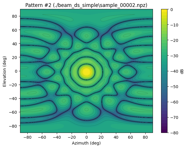
def visualize_samples(npz_files, db_floor=-80, title_prefix="Pattern"):

    for i, path in enumerate(npz_files):
        data = np.load(path, allow_pickle=True)
        pat_db = data["pattern_db"]
        az_plot = data["az_plot"]
        el_plot = data["el_plot"]

        plot_pattern_2d(
            az_plot, el_plot, pat_db,
            db_floor=db_floor,
            title=f"{title_prefix} #{i} ({path})"
        )
paths = generate_and_save(n=5, save_dir="./beam_ds_simple", seed=123)

visualize_samples(paths[:3], db_floor=-80)
.png)
.png)
The AI Network Model
To synthesize patterns using deep learning, we create a convolutional neural network. The radiation pattern is defined in the range of azimuth and elevation angle. Thus, this diagram can be represented as an image that our input layer accepts as input data. The output data are the weights that form such a diagram.
class ResNet18Beamformer(nn.Module):
    def __init__(self, num_outputs, in_channels=1):
        super().__init__()
        self.model = models.resnet18(weights=None)
        if in_channels == 1:
            conv1 = self.model.conv1
            self.model.conv1 = nn.Conv2d(
                1, conv1.out_channels,
                kernel_size=conv1.kernel_size, stride=conv1.stride,
                padding=conv1.padding, bias=False
            )
        self.model.fc = nn.Linear(self.model.fc.in_features, num_outputs)

    def forward(self, x): return self.model(x)
We will define the device on which the model is trained, as well as initialize the model itself. We will immediately transfer the model to the GPU
device = torch.device('cuda' if torch.cuda.is_available() else 'cpu')

model = ResNet18Beamformer(num_outputs=2*N, in_channels=1).to(device)
The data loader
Creating data loaders
class RadarPatternNPZ(Dataset):
    def __init__(self, files, db_floor=DB_FLOOR, resize=IMAGE_SIZE):
        self.files = files
        self.db_floor = float(db_floor)
        self.resize = int(resize)

        self.transform = transforms.Compose([
            transforms.Resize((self.resize, self.resize), interpolation=Image.BILINEAR),
            transforms.ToTensor(),
            transforms.Normalize([0.5], [0.5]),
        ])

    def __len__(self): return len(self.files)

    def __getitem__(self, idx):
        path = self.files[idx]
        npz = np.load(path, allow_pickle=True)
        pat_db = npz["pattern_db"]
        img_u8 = db_to_uint8(pat_db, self.db_floor)
        img = Image.fromarray(img_u8, mode="L")
        x = self.transform(img)

        w = npz["weights"].astype(np.complex64)

        w = normalize_weights(w)
        y = np.stack([w.real, w.imag], axis=1).astype(np.float32).ravel()
        y = torch.from_numpy(y)
        return x, y, path

def make_loaders(root_dir=SAVE_DIR, batch_size=BATCH_SIZE, seed=SEED):
    files = sorted(glob.glob(os.path.join(root_dir, "sample_*.npz")))
    if not files: raise FileNotFoundError("No .npz in " + root_dir)
    gen = torch.Generator().manual_seed(seed)
    n = len(files)
    n_train = int(0.7 * n)
    n_val   = int(0.15 * n)
    n_test  = n - n_train - n_val
    idx_train, idx_val, idx_test = random_split(range(n), [n_train, n_val, n_test], generator=gen)
    train_ds = RadarPatternNPZ([files[i] for i in idx_train.indices])
    val_ds   = RadarPatternNPZ([files[i] for i in idx_val.indices])
    test_ds  = RadarPatternNPZ([files[i] for i in idx_test.indices])
    return (
        DataLoader(train_ds, batch_size=batch_size, shuffle=True,  num_workers=0),
        DataLoader(val_ds,   batch_size=batch_size, shuffle=False, num_workers=0),
        DataLoader(test_ds,  batch_size=batch_size, shuffle=False, num_workers=0),
        files
    )
Some auxiliary functions for network training and validation
Let's define the functions responsible for training and validation
def train_one(model, loader, criterion, optimizer, device, amp_dtype=None):
    model.train()
    run_loss, run_mae, n = 0.0, 0.0, 0
    for xb, yb, _ in loader:
        xb, yb = xb.to(device, non_blocking=True), yb.to(device, non_blocking=True)
        bs = xb.size(0)
        optimizer.zero_grad(set_to_none=True)
        with torch.autocast(device_type=device.type, dtype=amp_dtype) if amp_dtype else torch.cuda.amp.autocast(enabled=False):
            yp = model(xb)
            loss = criterion(yp, yb)
        loss.backward(); optimizer.step()
        run_loss += loss.item() * bs
        run_mae  += torch.mean(torch.abs(yp.detach() - yb)).item() * bs
        n += bs
    return run_loss/max(1,n), run_mae/max(1,n)

@torch.no_grad()
def evaluate(model, loader, criterion, device, amp_dtype=None):
    model.eval()
    run_loss, run_mae, n = 0.0, 0.0, 0
    for xb, yb, _ in loader:
        xb, yb = xb.to(device), yb.to(device)
        bs = xb.size(0)
        with torch.autocast(device_type=device.type, dtype=amp_dtype) if amp_dtype else torch.cuda.amp.autocast(enabled=False):
            yp = model(xb)
            loss = criterion(yp, yb)
        run_loss += loss.item() * bs
        run_mae  += torch.mean(torch.abs(yp - yb)).item() * bs
        n += bs
    return run_loss/max(1,n), run_mae/max(1,n)

def train_model(model, train_loader, val_loader, device, epochs=EPOCHS, lr=LR, wd=WEIGHT_DECAY):
    criterion = nn.MSELoss()
    optimizer = torch.optim.AdamW(model.parameters(), lr=lr, weight_decay=wd)
    amp_dtype = torch.bfloat16 if device.type == "cuda" else None

    best_wts = copy.deepcopy(model.state_dict())
    best_val = float("inf")
    for ep in range(1, epochs+1):
        tr_loss, tr_mae = train_one(model, train_loader, criterion, optimizer, device, amp_dtype)
        val_loss, val_mae = evaluate(model, val_loader, criterion, device, amp_dtype)
        if val_loss < best_val:
            best_val, best_wts = val_loss, copy.deepcopy(model.state_dict())
        print(f"Epoch {ep:02d}/{epochs} | train: loss {tr_loss:.5f}, mae {tr_mae:.5f} | val: loss {val_loss:.5f}, mae {val_mae:.5f}")
    model.load_state_dict(best_wts)
    return model
Function for inference
@torch.no_grad()
def predict_weights(model, pat_db, device):
    # the same preprocessing as in the dataset
    img_u8 = db_to_uint8(pat_db, DB_FLOOR)
    img = Image.fromarray(img_u8, mode="L")
    tfm = transforms.Compose([
        transforms.Resize((IMAGE_SIZE, IMAGE_SIZE), interpolation=Image.BILINEAR),
        transforms.ToTensor(),
        transforms.Normalize([0.5],[0.5]),
    ])
    x = tfm(img).unsqueeze(0).to(device)
    y = model(x).cpu().numpy().reshape(-1,2)
    w_pred = y[:,0] + 1j*y[:,1]
    w_pred = normalize_weights(w_pred)   # fixing the uncertainties
    return w_pred
Model training
Let's divide the data into three sets - training, test, and validation
We will also define the potel function, an optimizer for network training, and run the training cycle itself.
train_loader, val_loader, test_loader, files = make_loaders(SAVE_DIR, BATCH_SIZE, SEED)
print(f"Train/Val/Test sizes: {len(train_loader.dataset)}/{len(val_loader.dataset)}/{len(test_loader.dataset)}")
    # 3) the model

criterion = nn.MSELoss()
optimizer = torch.optim.AdamW(model.parameters(), lr=LR, weight_decay=WEIGHT_DECAY)
amp_dtype = torch.bfloat16 if device.type == "cuda" else None

best_wts = copy.deepcopy(model.state_dict())
best_val = float("inf")
for ep in range(1, EPOCHS+1):
    tr_loss, tr_mae = train_one(model, train_loader, criterion, optimizer, device, amp_dtype)
    val_loss, val_mae = evaluate(model, val_loader, criterion, device, amp_dtype)
    if val_loss < best_val:
        best_val, best_wts = val_loss, copy.deepcopy(model.state_dict())
    print(f"Epoch {ep:02d}/{EPOCHS} | train: loss {tr_loss:.5f}, mae {tr_mae:.5f} | val: loss {val_loss:.5f}, mae {val_mae:.5f}")
model.load_state_dict(best_wts)
print(f"Train/Val/Test sizes: {len(train_loader.dataset)}/{len(val_loader.dataset)}/{len(test_loader.dataset)}")
Testing a trained model
Let's make an assessment on the test set of the trained model.
crit = nn.MSELoss()
val_loss, val_mae = evaluate(model, test_loader, crit, device)
print(f"Test  : loss {val_loss:.6f}, mae {val_mae:.6f}")
Let's test the model on a newly generated data instance.
interfs = [(12.0, 10.0), (13.0, 10.0)]
interfs_db = [-30.0, -30.0]
az_bands = [(-20, -10), (10, 20)]
el_bands = [(-20, -10), (10, 20)]
exclude = set(interfs)
side_pts = []
for az_span in az_bands:
for el_span in el_bands:
side_pts += make_side_region(az_span, el_span, step=0.5, exclude=exclude)
w_ref = synthesize_mask_l2(pos, (0.0,0.0), interfs, interfs_db, side_pts, -17.0)
w_ref = normalize_weights(w_ref)
pat_ref = array_response_fast(pos, w_ref, az_plot, el_plot)
w_pred_new = predict_weights(model, pat_ref, device)
pat_pred_new = array_response_fast(pos, w_pred_new, az_plot, el_plot)
plot_pattern_cut(az_plot, el_plot, pat_ref, el0=0.0, title="The standard")
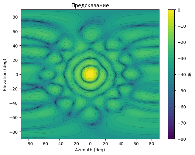
plot_pattern_cut(az_plot, el_plot, pat_pred_new, el0=0.0, title="Prediction")
plot_pattern_2d(az_plot, el_plot, pat_ref, db_floor=-80, title='The standard')
plot_pattern_2d(az_plot, el_plot, pat_pred_new, db_floor=-80, title='Prediction')
.png)
.png)
.png)
In general, the model provides an acceptable quality on the inference.
Conclusions
This example showed how to generate directional patterns and use them to train a model for predicting weights.