A generative network for synthesizing signals

This example shows how a generative neural network (GAN) can be used to synthesize realistic radar signals. This can be useful for increasing the training sample, modeling scenarios, or generating data with limited access to real-world measurements.

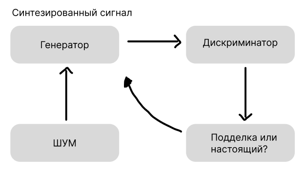
A generative-adversarial network is two neural networks in which a generator takes a noise signal as input and tries to make a plausible signal out of it, and the discriminator receives either this synthesized signal or a real one and learns to distinguish a fake from reality by transmitting an error to the generator so that it becomes better at masking its fakes over time.

The generator receives noise as a one-dimensional signal from a random distribution and transforms it through a chain of neural network layers into a synthesized signal, which outwardly should strive to be similar to the real signal.

The discriminator receives either a synthesized signal from the generator or a real signal from the training set as input. After that, it passes it through its own network to decide whether it is real or fake, and issues a probability estimate.

Based on this estimate, the error is calculated for both parts of the system and the generator learns to improve its syntheses in order to deceive the discriminator. The discriminator learns to more accurately distinguish a fake from a real signal. As they learn, both ANNs improve their abilities and over time, the synthesized signal becomes almost indistinguishable from the real one.

Importing the necessary packages for work

include("$(@__DIR__)/InstallPackages.jl")

using Pkg
Pkg.instantiate()
using Glob
using DSP
using CUDA
using Flux 
using Statistics
using cuDNN
using BSON: @save, @load 
using Zygote

Since the functions used have a fairly large number of lines of code, they have been moved to separate files.jls that are imported below
The model.jl file implements the structure of the model used. The dataset.jl file is used to implement the logic of the dataset module.

Dirpath = "$(@__DIR__)"
include(joinpath(Dirpath, "model.jl"))
include(joinpath(Dirpath, "dataset.jl"))

Creating a data loader

Next, we will create a data loader that will load data into the model in batches. In the block below, we will initialize the dataset.
The dataset logic is written in the dataset.jl file
The dataset slices the ECG and radar signal onto the overlaid windows. Slicing allows you to reduce the load on the ANN due to the use of long sequences, and the use of overlap allows you to take into account time dependencies.

function mycollate(batch)
    radar = hcat(first.(batch)...)           
    ecg   = hcat(last.(batch)...)          
    return radar, ecg
end

mycollate (generic function with 1 method)

ds = RadarECG("prepareRadarData");
N = length(ds)
train_idx = 1:N
X_train = [ ds[i][1] for i in train_idx ]  
Y_train = [ ds[i][2] for i in train_idx ]    
batch_size = 64
train_loader = Flux.DataLoader((X_train, Y_train);
    batchsize = batch_size,
    shuffle   = true,
    partial      = true,
    parallel = true,
    collate   = mycollate
);

After that, we will determine the device on which the model will be trained. If you have access to a GPU, training will be accelerated by several orders of magnitude. We will also transfer the data loader to the device we are using.

device = CUDA.functional() ? gpu : cpu;
device == gpu ? train_loader = gpu.(train_loader) : nothing;

Initializing models

Next, we initialize the ANN generator and discriminator, and also define the optimizers used, in this case, Adam.

nz = 100
net_G = Generator(nz)
net_D = Discriminator()
    
net_G = gpu(net_G)
net_D = gpu(net_D);

η_D, η_G = 5e-5, 2e-4
optD = Adam(η_D, (0.5, 0.999))            # без WeightDecay
optG = Adam(η_G, (0.5, 0.999));

Let's define the path where the trained models will be saved.

isdir("output")||mkdir("output")
Dirpath = "$(@__DIR__)"
train_path = joinpath(Dirpath, "output");

Model training

Let's define the functions that perform GAN training, as well as loss functions for each of the subnets - the generator and the discriminator.

function discr_loss(real_output, fake_output)
    real_loss = Flux.logitbinarycrossentropy(real_output, 1f0)
    fake_loss = Flux.logitbinarycrossentropy(fake_output, 0f0)
    return (real_loss + fake_loss) / 2
end



generator_loss(fake_output) = Flux.logitbinarycrossentropy(fake_output, 1f0)

function train_discr(discr, original_data, fake_data, opt_discr)
    ps = Flux.params(discr)
    loss, back = Zygote.pullback(ps) do
                      discr_loss(discr(original_data), discr(fake_data))
    end
    grads = back(1f0)
    Flux.update!(opt_discr, ps, grads)
    return loss
end

Zygote.@nograd train_discr

function train_gan(gen, discr, original_data, opt_gen, opt_discr, nz, bsz)
    noise = randn(Float32, 2, nz, bsz) |> gpu
    loss = Dict()
    ps = Flux.params(gen)
    loss["gen"], back = Zygote.pullback(ps) do
                          fake_ = gen(noise)
                          loss["discr"] = train_discr(discr, original_data, fake_, opt_discr)
                          generator_loss(discr(fake_))
    end
    grads = back(1f0)
    Flux.update!(opt_gen, ps, grads)
    return loss
end

train_gan (generic function with 1 method)

Let's start the training

train_steps = 0
epochs = 100
verbose_freq = 40
for ep in 1:epochs
    @info "Epoch $ep"
    for (i, (radar, _)) in enumerate(train_loader)
        radar = reshape(radar, size(radar,1), 1, size(radar,2)) |> gpu
        radar .+= 0.05f0 .* randn(Float32, size(radar)) |> gpu 
        loss = train_gan(net_G, net_D, radar, optG, optD, nz, batch_size)
        if train_steps % verbose_freq == 0
            noiseZ = randn(Float32,2,nz, batch_size) |> gpu
            P_real = mean(sigmoid.(net_D(radar)))
            P_fake = mean(sigmoid.(net_D(net_G(noiseZ))))
            @info("[$ep/$(epochs)] step $train_steps  " *
                  "P(real)=$(round(P_real,digits=3))  " *
                  "P(fake)=$(round(P_fake,digits=3))")
        end
        train_steps += 1
    end
end

Next, we will save the trained models

# Переносим модели на CPU
train_dir = joinpath(Dirpath, "output")
net_D_cpu = cpu(net_D)
net_G_cpu = cpu(net_G)

# Пути для сохранения
output_dir_D = joinpath(train_dir, "modelsD_bson")
output_dir_G = joinpath(train_dir, "modelsG_bson")

# создаём папки, если их нет
isdir(output_dir_D) || mkdir(output_dir_D)
isdir(output_dir_G) || mkdir(output_dir_G)

# имена файлов для лучших моделей
best_path_D = joinpath(output_dir_D, "discriminator.bson")
best_path_G = joinpath(output_dir_G, "generator.bson")

# сохраняем лучший дискриминатор
@info "Сохраняем дискриминатор в $best_path_D"
@save best_path_D net_D_cpu

# сохраняем лучший генератор
@info "Сохраняем генератор в $best_path_G"
@save best_path_G net_G_cpu

[ Info: Сохраняем дискриминатор в /user/Диплом/GANECG/output/modelsD_bson/discriminator.bson
[ Info: Сохраняем генератор в /user/Диплом/GANECG/output/modelsG_bson/generator.bson

Testing the model

Generate signals from the noise

noise = randn(Float32, 1, 100, 16) |> gpu
fake  = net_G(noise)
fakec = cpu(fake);
ind = 2
plot(fakec[:, 1, ind]/6)

Conclusions

In this demo example, the GAN neural network was trained to generate synthetic data based on real data.