Reading data from Excel format and building models
Very often, the data that needs to be analyzed is not taken from some abstract repositories or databases, but lies in some kind of tabular format file. In some industries, CSV is the preferred format; in other cases, data is created in standard tabular editors.
In this demo, we will learn how to load and display data from an Excel spreadsheet on a graph and build a model based on it.
Reading an entire file
For most commands, we will need the following libraries, which are already built into the environment. It only remains for us to indicate that we are going to use commands from the namespace of these libraries.
Pkg.add(["Interpolations", "XLSX", "GLM", "Optim"])
using XLSX, DataFrames
One Excel file can contain several sheets with tables. Most often, we use only the first of these sheets, which is called Лист1 or Sheet1 (but it may be called something else).
Reading the entire file will return us an object with several tables inside, each of which is located on a separate sheet.
xf = XLSX.readxlsx( "table_simple_example.xlsx" )
We can verify this again by displaying the list of sheets.
XLSX.sheetnames(xf)
If you have already opened the file with the command readxlsx then you can separate the desired sheet using an additional command.
sh = xf["Sheet 1"]
Or you can use commands that perform this process faster.
Reading a separate sheet from a table
Standards by library teams XLSX you can read each sheet individually.
XLSX.readtable( "table_simple_example.xlsx", "Sheet 1" )
You can put a sheet of the table in the format DataFrame and process the data using this library.
DataFrame( XLSX.readtable( "table_simple_example.xlsx", "Sheet 1" ) )
xdf = Float32.(DataFrame( XLSX.readtable( "table_simple_example.xlsx", "Sheet 1" ) ))
But it makes sense when the data is a set of objects and a list of their attributes. Sometimes the table contains just a matrix with numbers, and then it's better to work with it using a standard data type. Matrix.
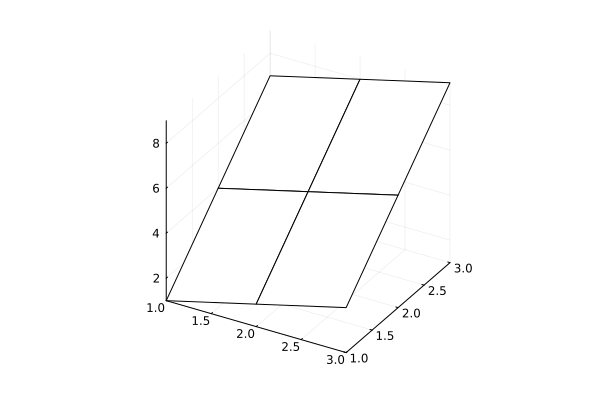
xm = XLSX.readdata( "table_simple_example.xlsx", "Sheet 1", "A2:C4" )
Choosing the right data type greatly simplifies further work with the table or matrix.
gr()
wireframe( xm )
Calculating data on a new computational grid (interpolation)
Now, we have at our disposal a table of data set in a certain coordinate system, we can perform their interpolation using a spline and build a model.
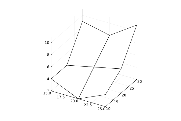
xm = vec( Float32.( XLSX.readdata("table_matrix_example.xlsx", "Sheet 1", "B1:D1") ))
ym = vec( Float32.( XLSX.readdata("table_matrix_example.xlsx", "Sheet 1", "A2:A4") ))
zm = Float32.( XLSX.readdata("table_matrix_example.xlsx", "Sheet 1", "B2:D4") )
wireframe( xm, ym, zm )
using Interpolations
# Converting the description of the coordinate system from vectors to a set of ranges
xSrc = range( minimum(xm), maximum(xm), step=xm[2]-xm[1] )
ySrc = range( minimum(ym), maximum(ym), step=ym[2]-ym[1] )
# We are building a model that will predict the values on the new grid.
cubInt = cubic_spline_interpolation( (xSrc, ySrc), zm )
# Setting a new calculation grid
xRange = range( minimum(xm), maximum(xm), 50 )
yRange = range( minimum(ym), maximum(ym), 50 )
zIntRes = cubInt(xRange, yRange)
# Visualize the result
surface( xRange, yRange, zIntRes, fillalpha=0.2 )
wireframe!( xRange, yRange, zIntRes )
We performed cubic spline interpolation. If the original data points were located in the coordinate system, but with irregular serifs along the X and Y axes, then we would only be able to build a model based on linear interpolation (or the "nearest neighbor method" model).
Function approximation and minimum search
After visual analysis of the data, you can make an assumption about which function would be convenient to approximate this data. This requires some experience and interactive work with the data.
Let's assume that we have made sure that the data is well represented using a quadratic function. Let's construct a polynomial that will allow us to more accurately find the estimated values of the output parameters in which the target value of the process under study is minimal.
using GLM
# Let's prepare the data: let's present the table as a list of individual data points
xx = Float64.(repeat( collect(xSrc), outer = length(ySrc) ))
yy = Float64.(repeat( collect(ySrc), inner = length(xSrc) ))
zz = Float64.(vec(reshape(zm', 1, :)))
# Creating a DataFrame object
data = DataFrame( X = xx, Y = yy, Z = zz )
# Let's build a model with two input parameters
model = lm( @formula(Z ~ X + Y + X^2 + Y^2 + X*Y), data )
# Setting a new calculation grid
dx = 2 * abs(maximum(xm) - minimum(xm))
dy = 2 * abs(maximum(ym) - minimum(ym))
xRange = range( minimum(xm) - dx, maximum(xm) + dx, 50 )
yRange = range( minimum(ym) - dy, maximum(ym) + dy, 20 )
# Visualize the result
xx = repeat( collect(xRange), outer = length(yRange) )
yy = repeat( collect(yRange), inner = length(xRange) )
zz = reshape( GLM.predict(model, (;X=xx,Y=yy)), length(xRange), :)
# Let's build graphs
surface( xRange, yRange, zz', fillalpha=0.2, xlabel="x", ylabel="y", zlabel="z" )
wireframe!( xRange, yRange, zz' )
Models created using GLM they take a point cloud as input (as you saw, we used data in the form of one-dimensional vectors Vector) and allow you to perform extrapolation without any additional settings.
Finding the minimum point
Both objects allow us to find the minimum point of the function, the description of which we obtained from the table.
using Optim
opt = optimize( x->GLM.predict( model,(;X=[x[1]],Y=[x[2]]) )[1], [0.0,0.0] )
(x_min, y_min) = Optim.minimizer( opt )
surface( xRange, yRange, zz', xlabel="x", ylabel="y", zlabel="z", c=:viridis, zcolor=zz' )
scatter!( [x_min], [y_min], [GLM.predict( model,(;X=[x_min],Y=[y_min]) )[1]],
camera = (30,50), legend=false, cbar=false )
We have received a graph where the minimum is marked.
Writing data to an Excel file
To save the analysis results to another Excel spreadsheet, use the following command:
XLSX.openxlsx( "table_write_example_1.xlsx", mode="w" ) do xf
# Let's put the matrix on the first sheet
XLSX.rename!( xf[1], "Sheet 1" )
xw = reshape(xx, 1, :) # Let's make matrices out of vectors
for ind in CartesianIndices(xw)
XLSX.setdata!( xf["Sheet 1"], XLSX.CellRef( ind[1], ind[2]+1 ), xw[ind])
end
yw = reshape(yy, :, 1)
for ind in CartesianIndices(yw)
XLSX.setdata!( xf["Sheet 1"], XLSX.CellRef( ind[1]+1, ind[2] ), yw[ind])
end
zw = zz
for ind in CartesianIndices(zw)
XLSX.setdata!( xf["Sheet 1"], XLSX.CellRef( ind[1]+1, ind[2]+1 ), zw[ind])
end
# We'll put the DataFrame on the second sheet.
XLSX.addsheet!( xf, "Sheet 2" )
XLSX.writetable!( xf["Sheet 2"], eachcol(xdf), names(xdf); anchor_cell=XLSX.CellRef("A1"))
end
Or, much shorter, to save DataFrame in a single-sheet table:
XLSX.writetable( "table_write_example_2.xlsx", xdf, overwrite=true )
To save objects Matrix or Vector The tabular format is much more commonly used CSV.
Conclusion
In this example, we learned how to read files in Excel tabular format. We converted them to different formats.:
- format
DataFramewhich is best suited for analyzing tabular data - format
Matrix, which allows you to work with a group of numbers from the source table as a matrix
We also demonstrated how to perform interpolation and approximation of data read from an Excel file and how to save the results.