Engee Graph Gallery
In this set of examples, we will show what the most diverse types of graphs look like in Engee, and by what means such a result is achieved – examples of data and code.
The right type of schedule allows you to save or convey the necessary information to the listener in a very eloquent, yet concise form. Graphs take information from variables that should exist in the memory workspace (_ should be visible in the Variables window_). They are usually displayed from interactive ngscript scripts, immediately after the corresponding code cells. Of course, there are exceptions.
- Unicode graphics can also be displayed on the command line, however, if interactive graphics are available, such a limited format may be needed only for the needs of special graphic design.;
- Graphs can be saved to file storage and opened as files from a file browser (sometimes useful).
The simplest and most frequently used command for displaying graphs is the function plot() from the library Plots for displaying graphs.
The Plots library in Engee is connected automatically.
At the same time, there are many more libraries in the Engee/Julia ecosystem for displaying beautiful graphs, some of which we will look at in this demo.:
StatsPlotsfor displaying complex statistical graphs,GMTorGeneral Mapping Toolsfor displaying geographical maps.
We also advise you not to avoid libraries that allow you to create much richer and more professional visualizations, for example:
Makiefor very high-quality visualization of complex data,Luxor– a language for creating vector two-dimensional graphics.
When the output library has built a graph, it transmits it to the graphical environment, and there are options here.:
- environment
gr(which is enabled by default) builds fast, economical and non-interactive graphs (enabled by the commandgr()), which can be saved using the context menu plotlyorplotlyjsthey create an interactive canvas on which the graph can be scaled, rotated and saved using the interface buttons (you can switch to them, respectively, with commandsplotly()andplotlyjs())
You can also choose a bitmap for displaying graphs (png) or vector (svg) format. By specifying inside the commands gr/plotly/plotlyjs argument fmt=:svg you will get a very elegant, scalable graph in vector format, however, if there are a large number of elements on the graph, especially if it is interactive, its output will require more resources. Raster graphics are another matter (fmt=:png). They build faster and do not require such resources when redrawing.
You will find the rest of the recipe elements for the perfect schedule below.
And now, we invite you to the graph gallery!
Pkg.add(["StatsPlots", "WordCloud", "MeshIO", "ColorSchemes", "Colors", "GMT", "Statistics", "StatsBase", "CSV", "Distributions", "Meshes"])
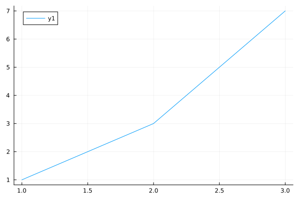
gr()
plot([1,2,3], [1,3,7])
Data analysis
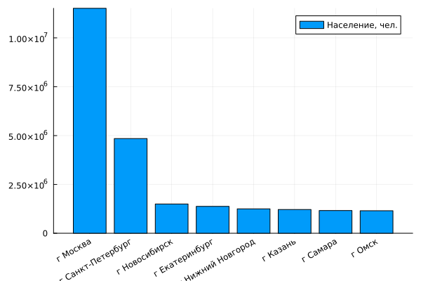
Building a bar chart based on a data table.
using DataFrames, HTTP, CSV;
# Open data from a file
data = sort( CSV.File( "data/city.csv" ) |> DataFrame, ["population"], rev=true );
# (or) Download data from the server
# url = "https://raw.githubusercontent.com/hflabs/city/master/city.csv"
# data = sort( CSV.File( HTTP.get(url).body) |> DataFrame, ["population"], rev=true );
bar( first(data, 8).population, label="Population, people", xrotation = 30 )
xticks!( 1:8, first(data, 8).address )
Studying the correlation of multidimensional data using the library StatsPlots and functions corrplor.
using StatsPlots, DataFrames, LaTeXStrings
M = randn( 1000, 4 )
M[:,2] .+= 0.8sqrt.(abs.(M[:,1])) .- 0.5M[:,3] .+ 5
M[:,3] .-= 0.7M[:,1].^2 .+ 2
corrplot( M, label = [L"$x_i$" for i=1:4],
xtickfontsize=4, ytickfontsize=6,
guidefontcolor=:blue, yguidefontsize=15, yguidefontrotation=-45.0 )
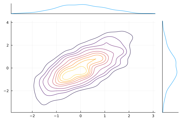
Function marginalkde from the library StatsPlots
using StatsPlots
x = randn(1024)
y = randn(1024)
marginalkde(x, x+y)
using DataFrames, Statistics
# Creating the data
df = DataFrame(Age=rand(4), Balance=rand(4), Position=rand(4), Salary=rand(4))
cols = [:Возраст, :Баланс, :Должность] # Let's select a part of the data
M = cor(Matrix(df[!,cols])) # The covariance matrix
# Chart
(n,m) = size(M)
heatmap( M, fc=cgrad([:white,:dodgerblue4]), xticks=(1:m,cols), xrot=90, yticks=(1:m,cols), yflip=true, leg=false )
annotate!( [(j, i, text(round(M[i,j],digits=3), 10,"Arial",:black)) for i in 1:n for j in 1:m] )
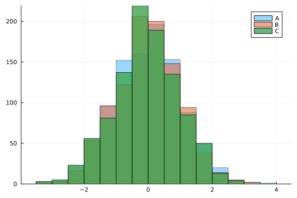
The usual histogram: function histogram
using Random
Random.seed!(2018)
x = randn(1000)
y = randn(1000)
z = randn(1000)
histogram(x, bins=20, alpha=0.4, label="A")
histogram!(y, bins=20, alpha=0.6, label="B")
histogram!(z, bins=20, alpha=0.8, label="C")
Two-dimensional sample distribution graph: function histogram2d
x = randn(10^4)
y = randn(10^4)
histogram2d(x, y)
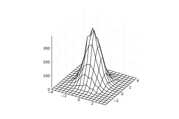
Volumetric graph of a two-dimensional histogram using wireframe
using StatsBase
x = randn(10^4)
y = randn(10^4)
h = StatsBase.fit( Histogram, (x, y), nbins=20 )
wireframe( midpoints(h.edges[1]), midpoints(h.edges[2]), h.weights )
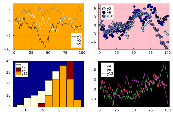
Combining schedules with different designs
using Random
Random.seed!(1)
plot( Plots.fakedata(100, 12),
layout = 4,
palette = cgrad.([:grays :blues :heat :lightrainbow]),
bg_inside = [:orange :pink :darkblue :black],
seriestype= [:line :scatter :histogram :line] )
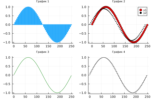
And just different types of graphs.:
x = 1:4:250;
y = sin.( 2pi/250 * x );
p1 = plot( x, y, title= "Schedule 1", seriestype=:stem, linewidth=3, legend=false )
p2 = plot( x, y, title= "Schedule 2", seriestype=:scatter, color=:red )
plot!( p2, x .- 10, 0.9y, seriestype=:scatter, color=:black, markersize=2 )
p3 = plot( x, y, title= "Schedule 3", seriestype=:line, color=:green, legend=false )
p4 = plot( x, y, title= "Schedule 4", seriestype=:steppre, color=:black, leg=false )
plot( p1, p2, p3, p4, layout=(2,2), titlefont=font(7), legendfont=font(7) )
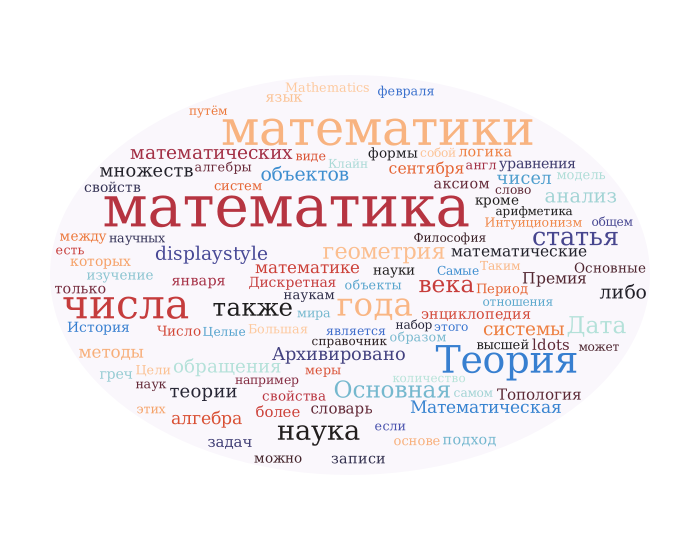
Wordcloud:
import Pkg; Pkg.add(["WordCloud"], io=devnull);
using WordCloud, HTTP
# Upload text from a file
content = read( open("data/Wikipedia - Математика.txt", "r"), String )
# Or download the data from the server
# url = "https://ru.wikipedia.org/wiki/Mathematics"
# resp = HTTP.request("GET", url, redirect=true)
# content = resp.body |> String |> html2text
stopwords = ["XVII", "that", "frac"];
stopwords = vcat(stopwords, string.(collect(1:100)));
wc = wordcloud( processtext( content, maxnum=100, stopwords=stopwords, minlength=4 ),
mask=shape(ellipse, 600, 400, color=(0.98, 0.97, 0.99), backgroundcolor=1, backgroundsize=(700, 550)),
masksize=:original, colors=:seaborn_icefire_gradient, angles=[0] ) |> generate!
paint(wc, "$(@__DIR__)/fromweb.svg")
wc
Animation
Creating GIF animations using the command @animate, which runs a third-party function in a loop that draws 150 circles of decreasing radius, with increasing transparency. Among others, you can also use the format mp4.
@userplot CirclePlot
@recipe function f(cp::CirclePlot)
x, y, i = cp.args
n = length(x)
inds = circshift(1:n, 1 - i)
linewidth --> range(0, 10, length = n)
seriesalpha --> range(0, 1, length = n)
aspect_ratio --> 1
label --> false
x[inds], y[inds]
end
n = 150
t = range(0, 2π, length = n)
x = sin.(t)
y = cos.(t)
anim = @animate for i ∈ 1:n
circleplot(x, y, i)
end
gif(anim, "$(@__DIR__)/anim_fps15.gif", fps = 15)
Rotating object (geometry is specified in the STL file)
import Pkg; Pkg.add(["Meshes", "MeshIO"], io=devnull);
using Meshes, MeshIO, FileIO
gr();
obj = load( "$(@__DIR__)/data/lion.stl" );
@gif for az in 0:10:359
p = plot( camera = (az, -20), axis=nothing, border=:none, aspect_ratio=:equal, size=(400,400) )
for i in obj
m = Matrix([i[1] i[2] i[3] i[1]])'
if m[1,1] > 0 plot!( p, m[:,1], m[:,2], m[:,3], lc=:green, label=:none, lw=.4, aspect=:equal )
else plot!( p, m[:,1], m[:,2], m[:,3], lc=:gray, label=:none, lw=.4, aspect=:equal )
end
end
end
Conclusion of matrices and images
Function heatmap
include( "$(@__DIR__)/data/peaks.jl" );
(x, y, z) = peaks()
heatmap(x, y, z)
using LaTeXStrings
x = range( -1.3, 1.3, 501 );
y = range( -1.3, 1.3, 501 );
X = repeat( x, outer = [1,501] )
Y = repeat( y', outer = [501,1] )
# C = ones( size(X) ) .* ( 0.360284 + 0.100376*1im );
C = ones( size(X) ) .* ( -0.75 + 0.1im );
Z_max = 1e6; it_max = 50;
Z = Complex.( X, Y );
B = zeros( size(C) );
for k = 1:it_max
Z = Z.^2 .+ C;
B = B .+ ( abs.(Z) .< 2 );
end
heatmap( B,
aspect_ratio = :equal,
cbar=false,
axis=([], false),
color=:jet )
title!( L"Julia Set $(c=0.360284+0.100376i)$" )
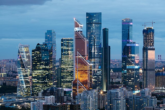
Output of illustrations from files: library Images
using Images
load( "$(@__DIR__)/data/640px-Business_Centre_of_Moscow_2.jpg" )
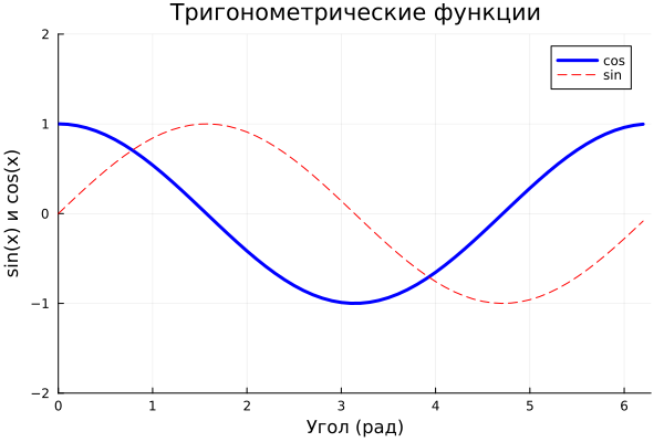
Graphs in Cartesian coordinates
Output of two trigonometric functions defined by vectors on a Cartesian coordinate plane.
x = 0:0.1:2pi
y1 = cos.(x)
y2 = sin.(x)
plot(x, y1, c="blue", linewidth=3, label="cos")
plot!(x, y2, c="red", line=:dash, label="sin")
title!("Trigonometric functions")
xlabel!("Angle (rad)")
ylabel!("sin(x) and cos(x)")
# Using a separate command, set the axis boundaries.
plot!( xlims=(0,2pi), ylims=(-2, 2) )
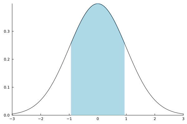
Filling in the area under the graph (argument fillrange)
using Distributions
x = range(-3, 3, 100 )
y = pdf.( Normal(0,1), x )
ix = abs.(x) .< 1
plot( x[ix], y[ix], fillrange = zero(x[ix]), fc=:blues, leg=false)
plot!( x, y, grid=false, lc=:black, widen=false )
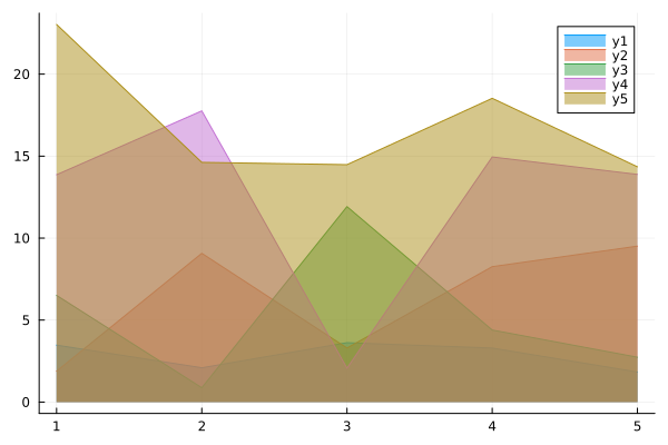
Schedule to fill in (area)
x = 1:10;
areaData = x .* rand(10,5) .* 5;
cur_colors = theme_palette(:default)
plot()
for i in 1:size(areaData,2)
plot!( areaData[i,:], fillcolor = cur_colors[i], fillrange = 0, fillalpha=.5 )
end
plot!()
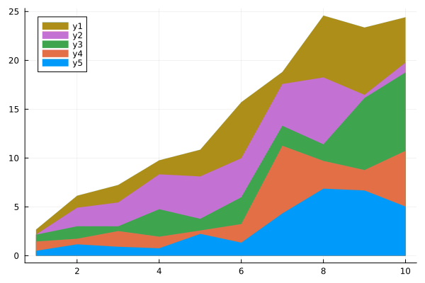
An accumulating schedule with filling in
x = 1:10;
areaData = x .* rand(10,5);
cur_colors = theme_palette(:default)
plot()
for i in size(areaData,2):-1:1
plot!( sum(areaData[:,1:i], dims=2), fillcolor = cur_colors[i], fillrange = 0, lw=0 )
end
plot!()
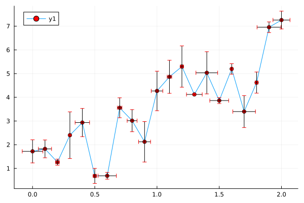
Graph with confidence intervals (arguments xerr and yerr)
using Random
Random.seed!(2018)
f(x) = 2 * x + 1
x = 0:0.1:2
n = length(x)
y = f.(x) + randn(n)
plot( x, y,
xerr = 0.1 * rand(n),
yerr = rand(n),
marker = (:circle, :red) )
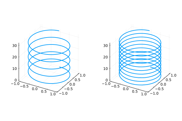
Three-dimensional graph
t = 0:pi/100:10pi;
x1 = sin.(1 * t)
y1 = cos.(1 * t)
x2 = sin.(2 * t)
y2 = cos.(2 * t)
plot(
plot( x1, y1, t, leg=false, lw=2 ),
plot( x2, y2, t, leg=false, lw=2 )
)
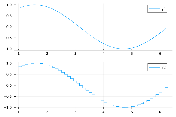
Smooth and stepwise graphs combined using an argument layout
x = range( 1, 2pi, length=50 )
plot( x, [sin.(x) sin.(x)],
seriestype=[:line :step],
layout = (2, 1) )
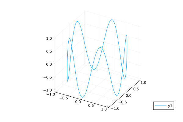
Parametric graph in 3D
t = range(0, stop=10, length=1000)
x = cos.(t)
y = sin.(t)
z = sin.(5t)
plot( x, y, z )
Graphs in polar coordinates
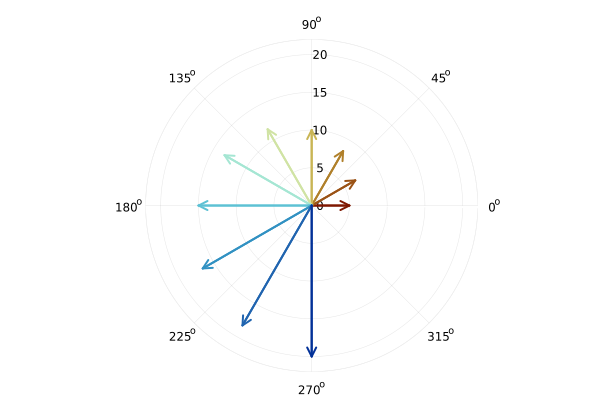
Arrows to the points forming the spiral (graph quiver)
cur_colors = theme_palette(:roma);
th = range( 0, 3*pi/2, 10 );
r = range( 5, 20, 10 );
c = collect(1:10)
X = r .* cos.(th)
Y = r .* sin.(th)
quiver( r.*0, r.*0, quiver=(th,r), aspect_ratio=:equal, proj=:polar,
line_z=repeat(c, inner=4), c=:roma, cbar=false, lw=2 )
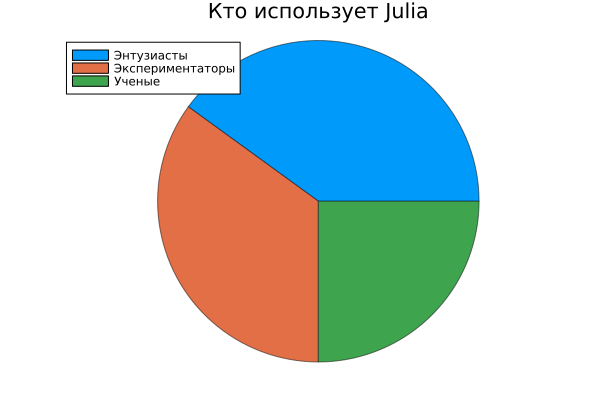
Function pie
x = [ "Enthusiasts", "The experimenters", "Scientists" ]
y = [0.4,0.35,0.25]
pie(x, y, title="Who uses Julia",l = 0.5)
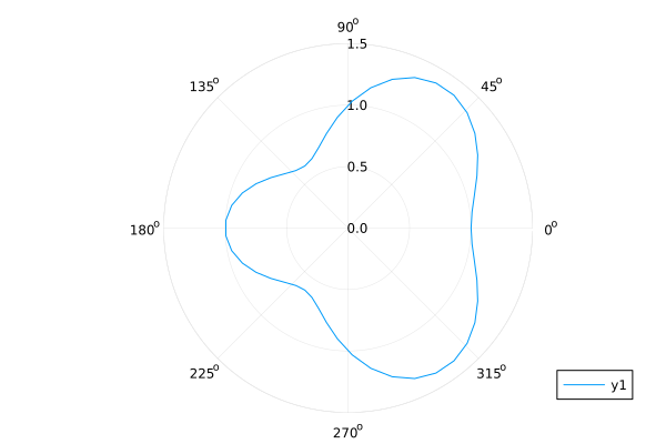
Function polar
θ = range(0, 2π, length=50)
r = 1 .+ cos.(θ) .* sin.(θ).^2
plot(θ, r, proj=:polar, lims=(0,1.5))
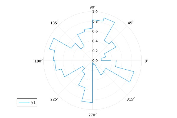
Stepwise graph in polar coordinates (graph rose)
using Random
Random.seed!(2018)
n = 24
R = rand(n+1)
θ = 0:2pi/n:2pi
plot( θ, R, proj=:polar, line=:steppre, lims=(0,1) )
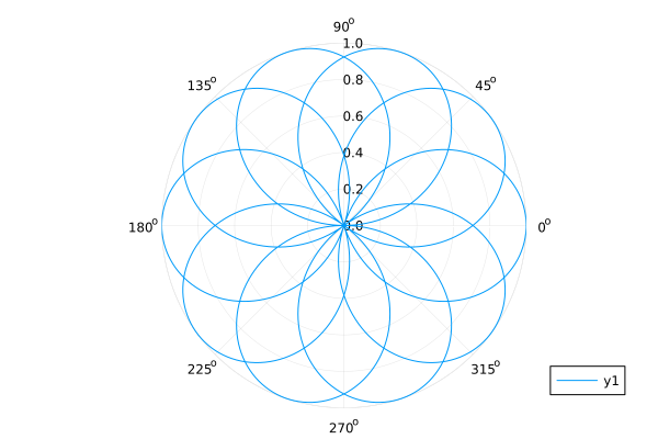
A graph in polar coordinates, set using the function
θ = range( 0, 8π, length=1000 )
fr(θ) = sin( 5/4 * θ )
plot( θ, fr.(θ), proj=:polar, lims=(0,1) )
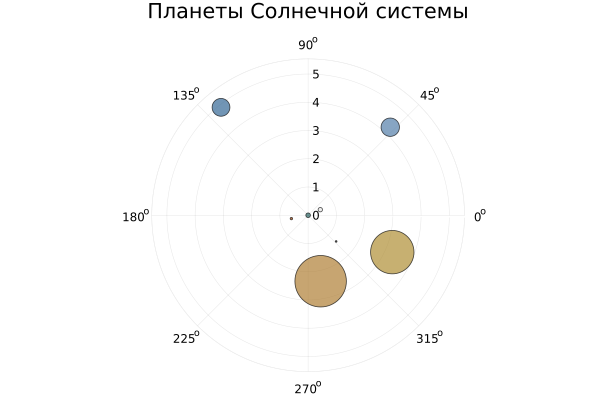
Bubble chart in polar coordinates
include( "$(@__DIR__)/data/planetData.jl" );
scatter( angle, distance, ms=diameter, mc = c,
proj=:polar, legend=false,
markerstrokewidth=1, markeralpha=.7 )
title!( "Planets of the Solar system" )
Discrete data
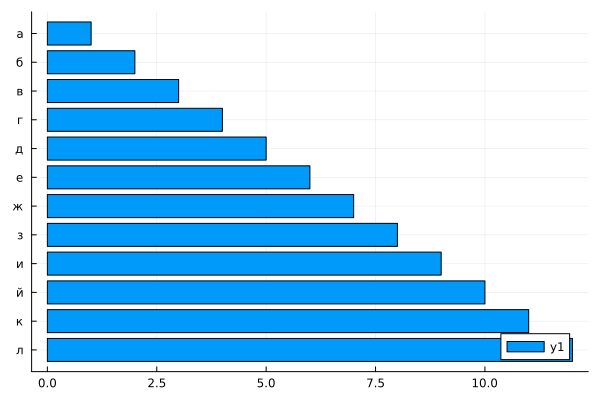
Horizontally positioned bar chart (function bar)
ticklabel = string.( collect('but':'m') )
bar( 1:12, orientation=:h, yticks=(1:12, ticklabel), yflip=true )
Bar charts bar and groupedbar
using StatsPlots
include( "$(@__DIR__)/data/BostonTemp.jl" );
plots_id = [1,2,3];
groupedbar( hcat([Temperatures[i,:] for i in plots_id]...),
xticks=(1:12, Months),
label = [Years[i] for i in plots_id]',
color = reshape(palette(:tab10)[1:3], (1,3)) )
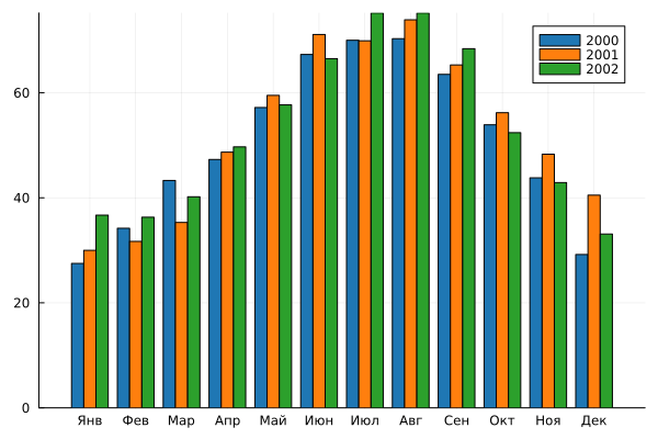
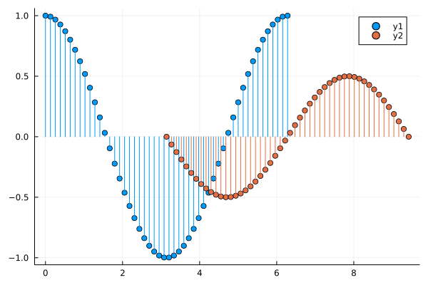
Chart stem (stvol-list)
x1 = range( 0, 2pi, 50 );
x2 = range( pi, 3pi, 50 );
X = [x1, x2];
Y = [cos.(x1), 0.5.*sin.(x2)];
plot( X, Y, line=:stem, marker=:circle )
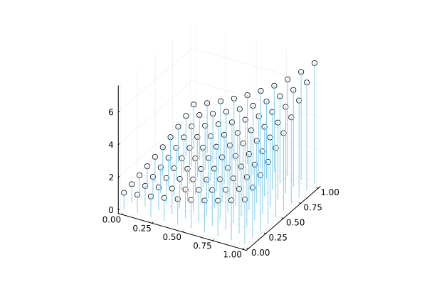
Three-dimensional stem-diagram
X = repeat( range(0,1,10), outer = [1,10] )
Y = repeat( range(0,1,10)', outer = [10,1] )
Z = exp.(X.+Y)
plot( X, Y, Z, line=:stem, color=:skyblue, markercolor=:white, marker=:circle, leg=false )
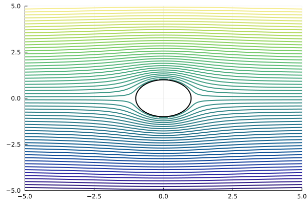
Contour graphs
Graph of laminar flow around a cylinder.
Analytical approximation of this function is calculated using the equation:
include( "$(@__DIR__)/data/flowAroundCylinder.jl" );
(r, theta, x, y, streamline, pressure) = flowAroundCylinder();
plot( x, y, streamline, levels=60, seriestype=:contour,
xlim = [-5,5], ylim=[-5,5], cbar=false, linewidth=2,
leg=false, color=:haline )
(xx,yy) = circle( 0, 0, 1 );
plot!( xx, yy, lw=2, lc=:black )
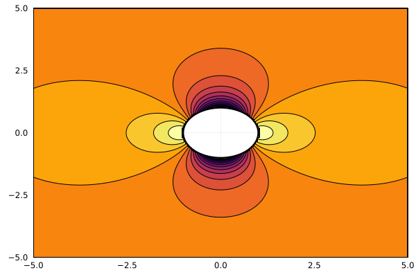
Filled contour graph (static pressure around a cylinder streamlined by a laminar flow)
include( "$(@__DIR__)/data/flowAroundCylinder.jl" );
(r, theta, x, y, streamline, pressure) = flowAroundCylinder();
plot( x, y, pressure, seriestype=:contourf, xlim = [-5,5], ylim=[-5,5], cbar=false, linewidth=1, leg=false )
(xx,yy) = circle( 0, 0, 1 );
plot!( xx, yy, lw=2, lc=:black )
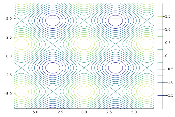
Contour graph of mathematical functions
# Prepare the data
y = x = range( -7, 7, step=0.1 )
z = @. sin(x) + cos(y')
Plots.contour( x, y, z, color=:haline )
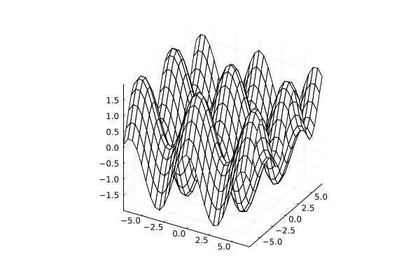
Surfaces and grids
Parameter seriestype=:surface
# Prepare the data
y = x = range( -7, 7, step=0.1 )
z = @. sin(x) + cos(y')
plot( x, y, z, st=:surface, color=:cool )
Parameter seriestype=:wireframe
# Prepare the data
y = x = range( -7, 7, step=0.5 )
z = @. sin(x) + cos(y')
plot( x, y, z, st=:wireframe )
Graph of a two-dimensional function
include( "$(@__DIR__)/data/peaks.jl" );
(x,y,z) = peaks();
plot( x, y, z; levels=20, st=:surface )
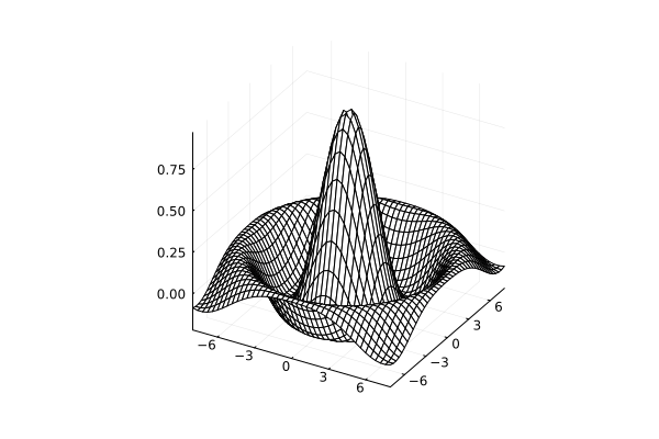
Let's plot the graph of the "sombrero" function. When using gr() argument hidesurface not used. But when using plotly() argument hidesurface=false allows you to simultaneously display both the surface and the contour graph on it.
x = y = range( -8, 8, length=41 )
f(x,y) = sin.(sqrt.(x.*x+y.*y))./sqrt.(x.*x+y.*y)
# in gr(), this method allows you to see the graph of the surface behind the graph of the lines.
p = plot( x, y, f, st=:surface, fillalpha=0.7, cbar=false )
plot!( p, x, y, f, st=:wireframe )
# plotly() has a more convenient syntax.
# wireframe( x, y, f, hidesurface=false )
A surface graph combined with a contour graph
Pkg.add("Contour")
using Contour
# Data
x = range(-3, 3, length=50)
y = range(-3, 3, length=50)
# z = [exp(-(xi^2 + yi^2)/5) * sin(xi^2 + yi^2) for xi in x, yi in y]
z = sin.(2*x) .+ cos.(1.6y')
colors = cgrad(:viridis, 8) # A palette of graphics divided into 10 colors
levels = range(minimum(z), maximum(z), length=10)[2:9] # 8 levels (from 2nd to 9th out of 10)
contour_data = Contour.contours(x, y, z, levels) # Contours with preset levels (many lines in each)
# Creating a 3D graph
surface(x, y, z, c=:viridis, legend=false) # 3D surface
# Contour graph on the XY plane
for cl in Contour.levels(contour_data)
lvl = level(cl) # the Z value of the contour
for line in lines(cl)
ys, xs = coordinates(line) # coordinates of the points of the current contour segment
plot!(xs, ys, zeros(size(xs)) .+ abs(1.1*minimum(z)), c=colors[lvl], lw=2)
end
end
plot!()
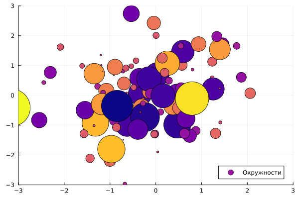
Dot charts and bubble charts
Bubble Chart
using Random: seed!
seed!(28)
xyz = randn(100, 3)
scatter( xyz[:, 1], xyz[:, 2], marker_z=xyz[:, 3],
label="Circles",
colormap=:plasma, cbar=false,
markersize=15 * abs.(xyz[:, 3]),
xlimits=[-3,3], ylimits=[-3,3]
)
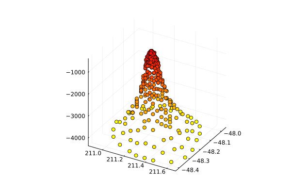
A three-dimensional dot graph with a separate color assigned to each point
using Colors, ColorSchemes
cs = ColorScheme([colorant"yellow", colorant"red"])

using CSV, DataFrames
df = DataFrame(CSV.File( "$(@__DIR__)/data/seamount.csv" ))
C = get( cs, df.z, :extrema )
scatter( df.x, df.y, df.z, c=C, leg=false )
A three-dimensional dot graph with a fictitious space for a color histogram
using CSV, DataFrames
df = DataFrame(CSV.File( "$(@__DIR__)/data/seamount.csv" ))
cs = cgrad(:thermal)
C = get( cs, df.x, :extrema )
l = @layout [a{0.97w} b]
p1 = scatter( df.x, df.y, df.z, c=C, leg=false )
p2 = heatmap(rand(2,2), clims=(0,10), framestyle=:none, c=cgrad(cs), cbar=true, lims=(-1,0))
plot(p1, p2, layout=l)
Color and annotations
Creating a color palette:
using Images
scheme = rand(RGB, 10)

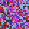
We use the palette to color the matrix from random numbers and output it as an image.:
matrix = rand(1:10, 20, 20)
img = scheme[ matrix ]
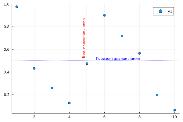
Let's create a graph from random points with lines and annotations.:
x = 1:10
y = rand(10)
# Creating a dot graph
scatter(x, y)
# Let's draw vertical and horizontal lines on the graph
vline!( [5], color=:red, linestyle=:dash, label=:none )
hline!( [0.5], color=:blue, linestyle=:dot, label=:none )
# Let's put annotations on the graph (it only works in gr())
annotate!( 8, 0.52, text("Horizontal line", :blue, :right, 8))
annotate!( 4.8, 0.7, text("Vertical line", :red, 8, rotation = 90))