Uploading data and processing passes
This example will demonstrate the process of downloading data from the XLSX format and filling in the gaps using the Impact and DataInterpolations libraries.
The data is an archive of observations of weather events at one weather station over the past 5 years.
In the example, only daily temperature measurements will be used.
Installing libraries necessary for downloading and processing data:
Pkg.add(["Statistics", "XLSX", "Impute", "CSV", "DataInterpolations"])
Pkg.add( "Impute" ); # loading the data processing library
Pkg.add( "DataInterpolations" );
Calling the libraries required for loading and processing data:
using DataFrames, CSV, XLSX, Plots, Impute, DataInterpolations, Statistics
using Impute: Substitute, impute
Reading data from a file to a variable:
xf_missing = XLSX.readxlsx("$(@__DIR__)/data_for_analysis_missing.xlsx");
Viewing sheet names in uploaded data:
XLSX.sheetnames(xf_missing)
Defining data from a file as a dataframe:
df_missing = DataFrame(XLSX.readtable("$(@__DIR__)/data_for_analysis_missing.xlsx", "data"));
Enabling a backend graphics display method:
gr()
Determination of variables characterizing the data - time and temperature:
x = df_missing.Time;
y = df_missing.T;
Plotting the temperature versus time dependence based on the initial data:
plot(x, y, labels="Temperature", title="Graph of temperature versus time")
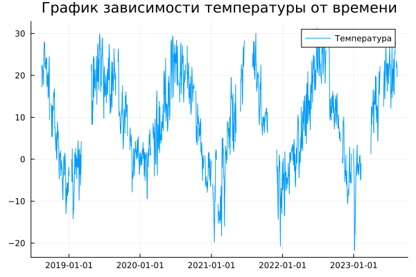
The graph shows that there are gaps in the data, they can be filled using the libraries Impact and DataInterpolations.
Using the Impact Library:
Defining a vector and a data matrix:
vectorT = df_missing[:,2]
matrixT = df_missing[:,1:2]
typeof(vectorT)
Converting vector and matrix to a format acceptable for the functions of the Impact library:
vectorT = convert(Vector{Union{Missing,Float64}}, vectorT);
matrixT[:,2] = convert(Vector{Union{Missing,Float64}}, matrixT[:,2]);
Filling in gaps using interpolation, filtering, and averages:
lin_inter_vectorT = Impute.interp(vectorT); # filling in missing values with interpolated ones (for signals)
filter_matrixT = Impute.filter(matrixT; dims=:rows); # deleting objects/observations with missing data
mean_matrixT = impute(matrixT[:,2], Substitute(; statistic=mean)); # filling in missing values with average values (suitable for statistical data)
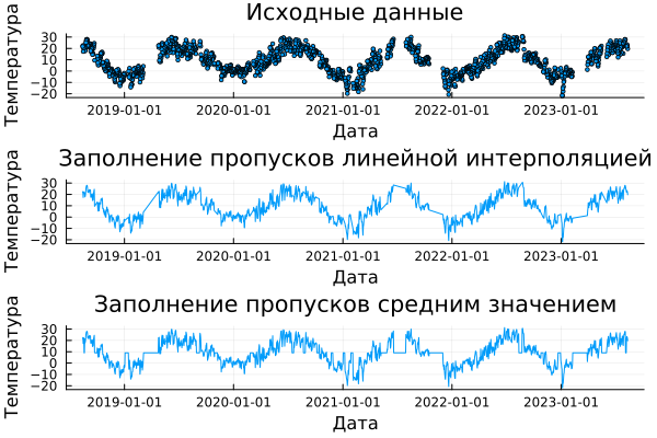
Plotting graphs with corrected data:
p2 = plot(df_missing[:,1], lin_inter_vectorT, xlabel="Date", ylabel="Temperature", title="Filling in gaps with linear interpolation", titlefont=font(10));
p3 = plot(df_missing[:,1], mean_matrixT, xlabel="Date", ylabel="Temperature", title="Filling in gaps with an average value", titlefont=font(10), guidefont=font(8));
p1 = scatter(df_missing[:,1], df_missing[:,2], markersize=2, xlabel="Date", ylabel="Temperature", title="Initial data", titlefont=font(10), guidefont=font(8))
plot(p1, p2, p3,  layout=(3, 1), legend=false)
Using the DataInterpolations Library
Data preparation for the use of interpolation methods:
days = [x for x in 1:length(df_missing[:,2])] # defining a vector from 1 to the length of the data array
t = days
u = reverse(df_missing[:,2]) # sorting temperature measurements in reverse order, from early to late
u = convert(Vector{Union{Missing,Float64}}, u); # converting data to the desired format for the methods used
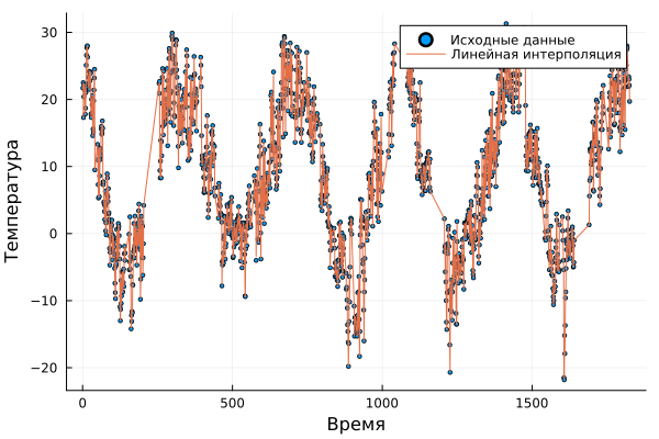
Filling in gaps using linear interpolation and plotting with corrected data:
A = LinearInterpolation(u,t)
scatter(t, u, markersize=2, label="Initial data") # output of a dot graph
plot!(A, label="Linear interpolation", xlabel="Time", ylabel="Temperature") # output of temperature versus time dependence
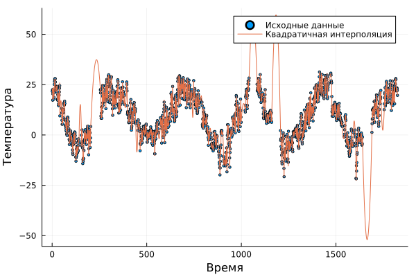
Filling in gaps using quadratic interpolation and plotting with corrected data:
B = QuadraticInterpolation(u,t)
scatter(t, u, markersize=2, label="Initial data")# output of a dot graph
plot!(B, label="Quadratic interpolation", xlabel="Time", ylabel="Temperature")# output of temperature versus time dependence
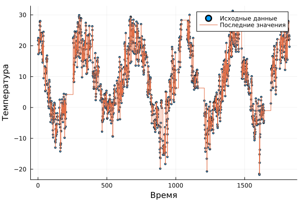
Filling in gaps by interpolating with the latest constant values and plotting with corrected data:
C = ConstantInterpolation(u,t)
scatter(t, u, markersize=2, label="Initial data")# output of a dot graph
plot!(C, label="Recent values", xlabel="Time", ylabel="Temperature")# output of temperature versus time dependence
Conclusion:
In this example, temperature measurement data was uploaded and preprocessed. Interpolation and filtering methods were applied.
According to the graphs obtained, it can be seen that some methods have limitations in their application to different types of data.
So, replacing omissions with an average value is more suitable for statistical analysis, where the characteristics of the data will not change much.
In the case of quadratic interpolation, there is a strong change in the magnitude of the signal in relatively large missing ranges, so that it is more applicable to small gaps.