Regression with neural network (minimal example)¶

In this example, we discuss the minimum number of operations required to train a fully-connected (fully-connected, FC) neural network on a regression task.

Task description¶

We will train the most classical kind of neural networks to "predict" the value of some one-dimensional function. Our goal is to compose the simplest algorithm, which we will later complicate (not the other way round).

Pkg.add(["Flux"])

# @markdown ## Настройка параметров нейросети
# @markdown *(двойной клик позволяет скрыть код)*
# @markdown
Параметры_по_умолчанию = false #@param {type: "boolean"}
if Параметры_по_умолчанию
    Коэффициент_скорость_обучения = 0.01
    Количество_циклов_обучения = 100
else
    Количество_циклов_обучения = 80 # @param {type:"slider", min:1, max:150, step:1}
    Коэффициент_скорость_обучения = 0.1 # @param {type:"slider", min:0.001, max:0.5, step:0.001}
end

epochs = Количество_циклов_обучения;
learning_rate = Коэффициент_скорость_обучения;

using Flux

Xs = Float32.( 0:0.1:10 );                    # Генерация данных для обучения
Ys = Float32.( Xs .+ 2 .* rand(length(Xs)) ); # <- ожидаемые от нейросети выходные данные
data = [(Xs', Ys')];                          # В таком формате данные передаются в функцию loss
model = Dense( 1 => 1 )                       # Архитектура нейросети: один FC-слой
opt_state = Flux.setup( Adam( learning_rate ), model ); # Алгоритм оптимизации
for i in 1:epochs
    Flux.train!( model, data, opt_state) do m, x, y
        Flux.mse( m(x), y ) # Функция потерь - ошибка на каждом элементе датасета
    end
end
X_прогноз = [ [x] for x in Xs ]               # Нейросеть принимает векторы, даже если у нас функция от одного аргумента
Y_прогноз = model.( X_прогноз )               # Для каждого [x] нейросеть вычисляет нам [y]

gr()                                          # Мы получили "вектор из векторов", который преобразуем для вывода на график
plot( Xs, Ys, label="Исходная выборка", legend=:topleft, lw=2 )
plot!( Xs, vec(hcat(Y_прогноз...)), label="Прогноз", lw=2 )

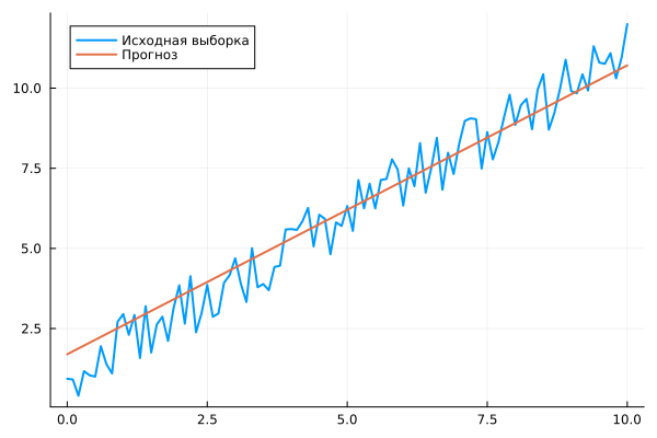
Change the parameters of the learning process and restart the cell using to evaluate how changing the settings would affect the quality of the forecast.

Creating a neural network as blocks on a canvas¶

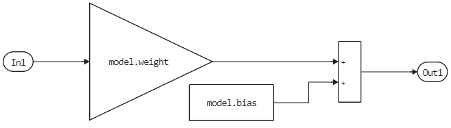
Our neural network has such a simple structure that it is very easy to transfer it "on canvas" and use it in your own library of blocks.

👉 This model can be run independently of the script. The "callbacks" of the model contain all the code for training the neural network, so when opening the file neural_regression_simple.engee for the first time, if the variable model does not exist yet, the neural network is trained again.

The model can be easily assembled from blocks in the workspace. It gets parameters from the variable workspace, but they can be entered into the properties of these blocks as fixed matrices and vectors.

Let's run this model and compare the results:

if "neural_regression_simple" ∉ getfield.(engee.get_all_models(), :name)
  engee.load( "$(@__DIR__)/neural_regression_simple.engee");
end

data = engee.run( "neural_regression_simple" );

# Поскольку в модели все операции у нас матричные, нам снова приходится "разглаживать" переменную Y
plot!( data["Y"].time, vec(hcat(data["Y"].value...)), label="Блок regression_net", lw=2 )

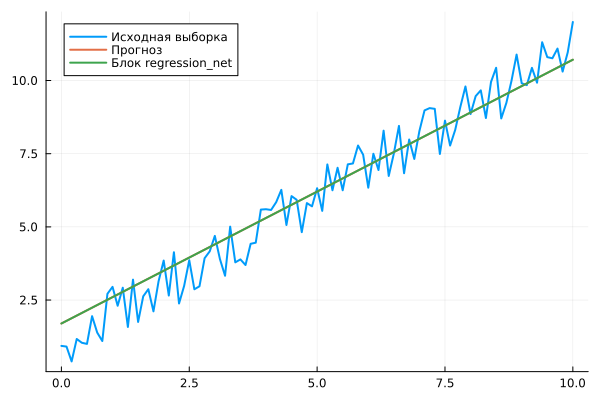
If the structure of the diagram is identical to that of the neural network, then the results of running "from code" and "from canvas" will also be identical.

Usually, the structure of a neural network changes less frequently than the data set and the problem formulation. Therefore, it is quite possible to model the structure twice: first in code, then as graphical blocks on the canvas.

Explanation of the code¶

Let's review our short code and comment on interesting points.

We use Float32 instead of Float64, which is the default in Julia (everything will work without it, but the Flux library will generate a single warning).

Xs = Float32.( 0:0.0.1:10 );
` Ys = Float32.(Xs .+ 2 .* rand(length(Xs)));

The accuracy of Float32 is more than enough for neural networks, their prediction errors usually exceed the rounding error due to the coarser bit grid. Plus, execution on the GPU, when we get to it, is faster with this type of data.

The data will be fed into the loss function via an iterator. Within the dataset, there should be tuples (Tuple) with columns of data - one column of inputs, one column of outputs. There are several other ways to feed the data, for now we will focus on the one below.

data = [(Xs', Ys')];

A neural network consists of a single element, a linear combination of inputs and weights with biases added (without an activation function, or, what is the same, with a linear activation function). We did not even surround the object Dense with the construct Chain(), which is usually used to create multilayer neural networks (although both ways, the network works the same way).

model = Dense( 1 => 1 )

Let's set up the Adam (Adaptive Moment Estimation) optimisation algorithm, one of the most effective optimisation algorithms in neural network training. The only parameter we pass to it is the learning rate coefficient.

opt_state = Flux.setup( Adam( learning_rate ), model_cpu )

** Now it's time to train the model.** We perform some number of repeated passes over the sample, compute the loss function and adjust all neural network variables in the direction of reducing the error gradient.

The loss function (loss function) is the only place where the model is explicitly executed during training. It is usually expressed through the sum of errors on each data item (the sum of cost functions). Here we simply use the standard mean squared error (MSE) function from the Flux library.

for i in 1:epochs
    Flux.train!(model, data, opt_state) do m, x, y
        Flux.mse( m(x), y )
    end
end

It remains to use the trained model. We pass input data to it as a function and get output predictions.

Y_forecast = model.( X_forecast )
X_forecast = [ [x] for x in Xs ]

Conclusion¶

We needed 10 lines of code to generate data and train the neural network, and another 5 to display its predictions on a graph. Small changes will allow you to make the neural network multilayer or train it on data from XLSX table.

We have found that once trained, it is quite easy to transfer the neural network to a canvas and use it as another block in the system diagram, and even generate C code from it if the diagram is simplified enough. In this way we can provide an end-to-end process of updating the system - from data sampling to the controller.

Regression with neural network (minimal example)¶

Task description¶

Creating a neural network as blocks on a canvas¶

Explanation of the code¶

Conclusion¶

Blocks used in example¶