Morphological operations, part 1
Morphological image processing is a field of computer vision that addresses the shortcomings of binary and grayscale images.
ImageMorphology contains a set of nonlinear operations related to the shape or morphology of image elements.
In this demo, we will look at the 8 most common morphological operations.
Pkg.add(["TestImages", "ImageMorphology"])
using Images
using ImageMorphology, TestImages
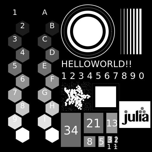
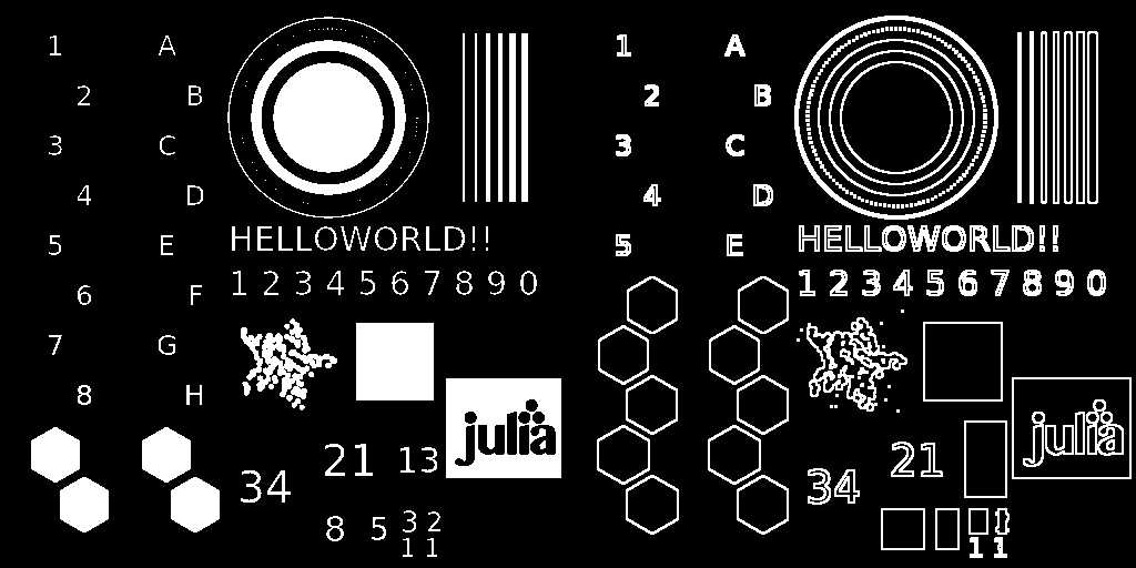
img = Gray.(testimage("morphology_test_512"))
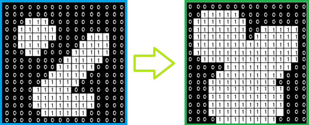
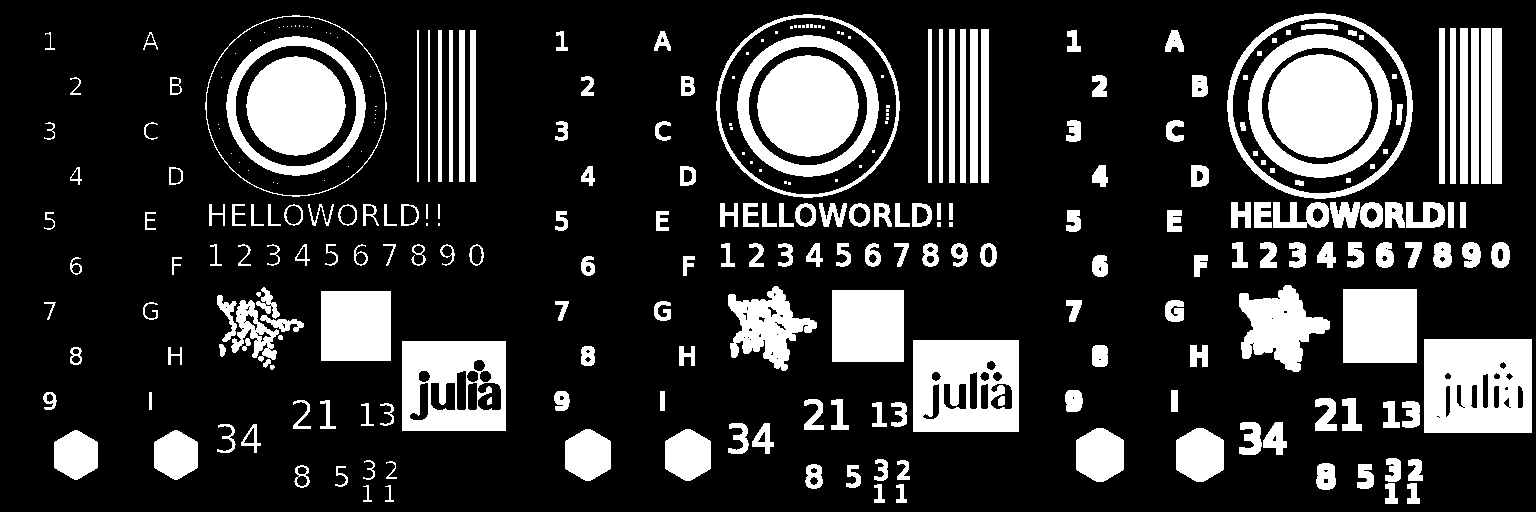
Erosion
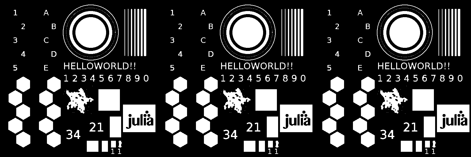
The erode function performs minimal filtering by nearest neighbors. By default, these are 8 links in 2d, 27 links in 3d, etc. You can specify a list of dimensions that you want to include in the connectivity, for example, region = [1,2] to exclude the third dimension from filtering.
Below is an example of how erosion works on a binary image using a 3x3 structuring element.
img_erode = @. Gray(img < 0.8); # keeps white objects white
img_erosion1 = erode(img_erode)
img_erosion2 = erode(erode(img_erode))
mosaicview(img_erode, img_erosion1, img_erosion2; nrow = 1)
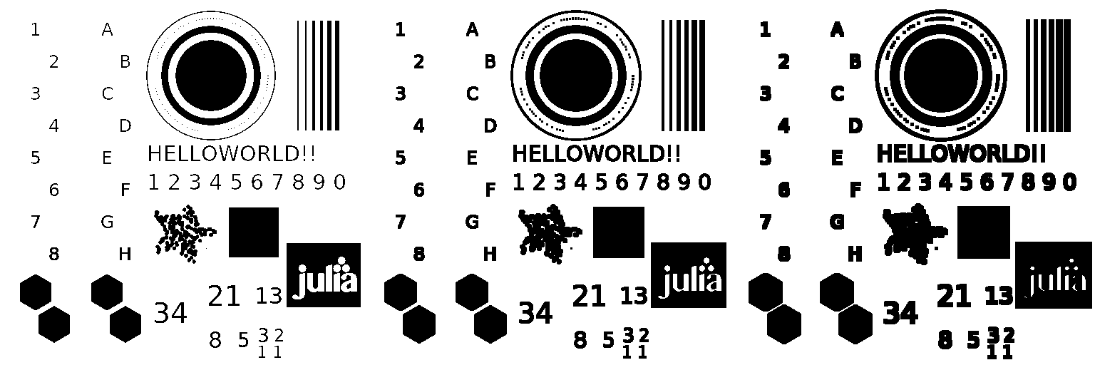
Expansion
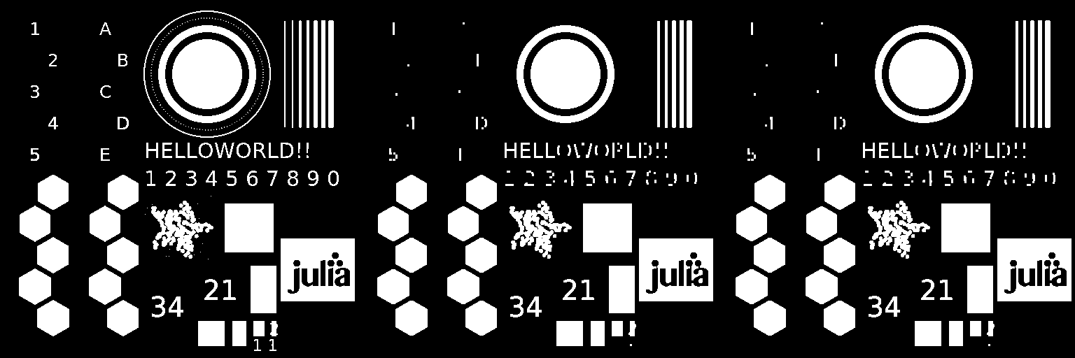
The dilate function performs maximizing filtering by its nearest neighbors. By default, it works the same way as erode.
.png)
img_dilate = @. Gray(img > 0.9);
img_dilate1 = dilate(img_dilate)
img_dilate2 = dilate(dilate(img_dilate))
mosaicview(img_dilate, img_dilate1, img_dilate2; nrow = 1)
Discovery
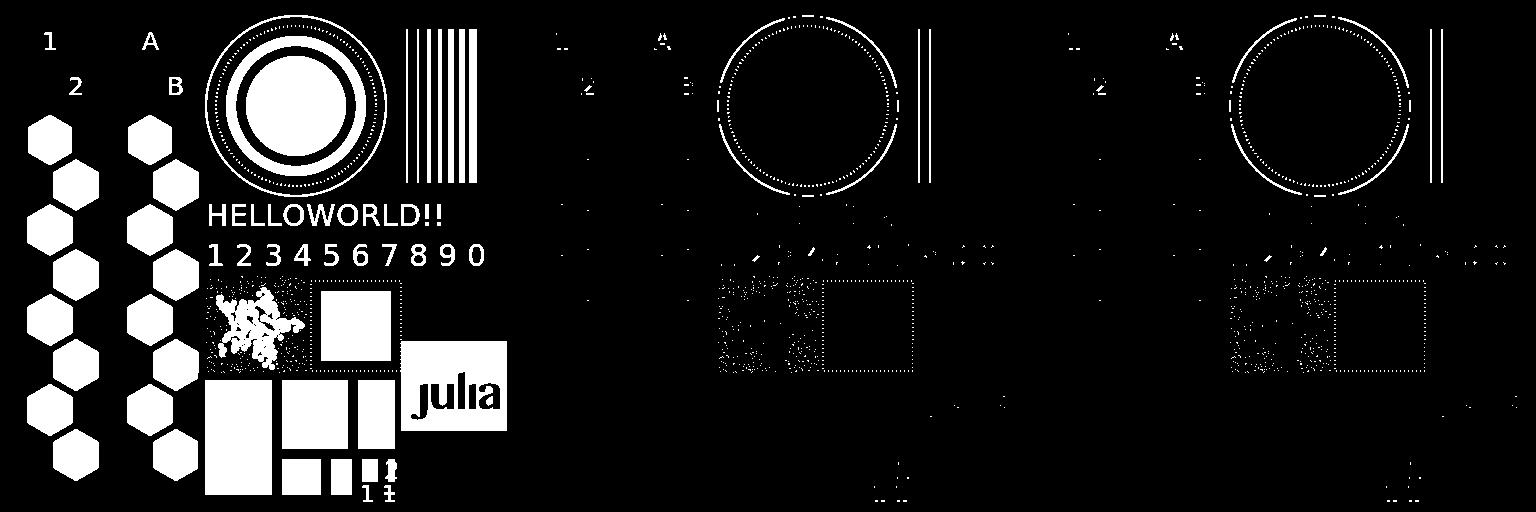
The opening morphology operation is equivalent to dilate(erode(img)). In the opening(img, [region]) function, region allows you to control the sizes over which this operation is performed.
Opening can remove small bright spots and connect small dark cracks.
img_opening = @. Gray(1 * img > 0.5);
img_opening1 = opening(img_opening)
img_opening2 = opening(opening(img_opening))
mosaicview(img_opening, img_opening1, img_opening2; nrow = 1)
Closure
Closing a morphology operation is equivalent to erode(dilate(img)). The closing(img, [region]) function works similarly to opening. Closing can remove small dark spots and connect small light cracks.
img_closing = @. Gray(1 * img > 0.5);
img_closing1 = closing(img_closing)
img_closing2 = closing(closing(img_closing))
mosaicview(img_closing1, img_closing1, img_closing2; nrow = 1)
Top-hat
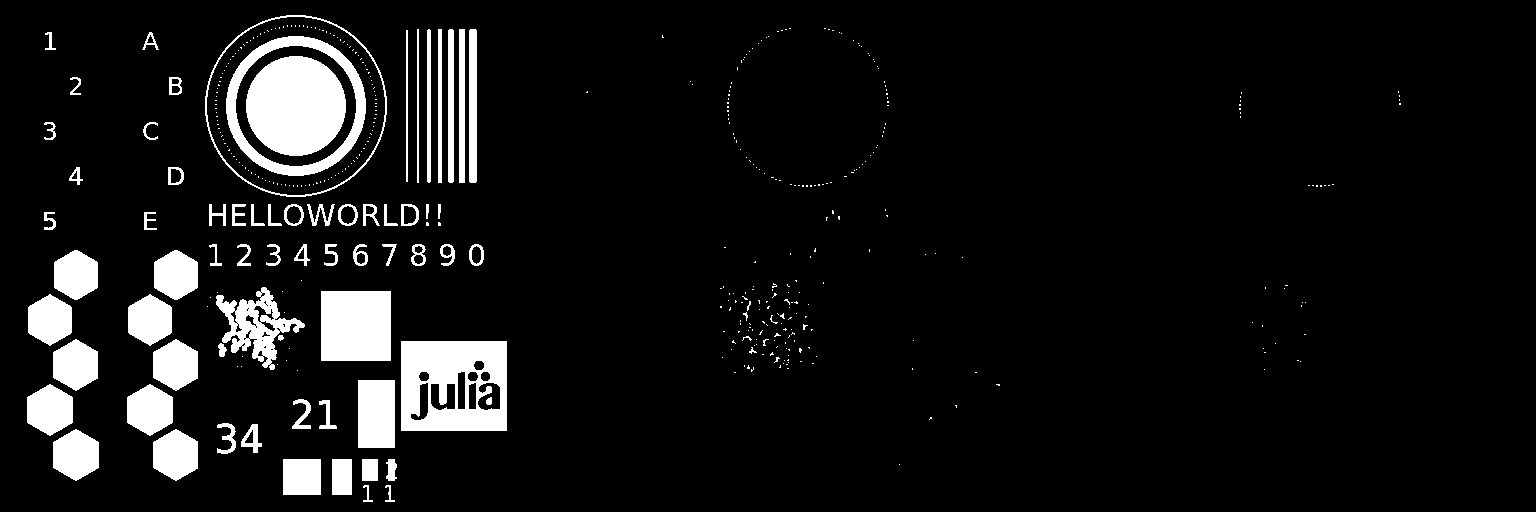
The tophat function is defined as an image minus its morphological opening. tophat(img, [region]) works similarly to opening and closing. This operation returns the bright spots of the image that are smaller than the structuring element.
img_tophat = @. Gray(1 * img > 0.2);
img_tophat1 = tophat(img_tophat)
img_tophat2 = tophat(tophat(img_tophat))
mosaicview(img_tophat, img_tophat1, img_tophat2; nrow = 1)
Bottom-Hat
The Bottom-Hat morphology operation is defined as the morphological closure of an image minus the original image. bothat(img, [region]) is defined similarly to tophat. This operation returns dark spots in the image that are smaller than the structuring element.
img_bothat = @. Gray(1 * img > 0.5);
img_bothat1 = bothat(img_tophat)
img_bothat2 = bothat(bothat(img_tophat))
img_bothat3 = bothat(bothat(bothat(img_tophat)))
mosaicview(img_bothat, img_bothat1, img_bothat2; nrow = 1)
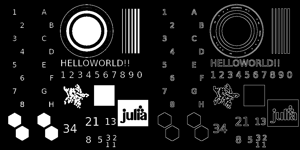
Morphology gradient
The morphological gradient is the difference between image expansion and erosion. morphogradient(img, [region]) is defined in the same way as tophat.
img_gray = @. Gray(0.8 * img > 0.7);
img_morphograd = morphogradient(@. Gray(0.8 * img > 0.4))
mosaicview(img_gray, img_morphograd; nrow = 1)
Morphological Laplace operator
The morphological Laplace operator returns a value, which is defined as the arithmetic difference between the inner and outer gradients. The morpholaplace(img, [region]) function is defined similarly to tophat.
img_gray = @. Gray(0.8 * Gray.(img) > 0.7);
img_morpholap = morpholaplace(img_gray)
mosaicview(img_gray, img_morpholap; nrow = 1)
Conclusion
In this example, we have analyzed some morphological operations that can be applied to images.