Visualization of drone instrument readings
In this example, algorithms for visualizing
flight data recorded from drone sensors are implemented.
The purpose of this demonstration is to show the various possibilities
of displaying data, including their time reference.
Let's start by reading the recorded data from the CSV file.
using CSV

# Reading data from the data.csv file
df_read = CSV.read("$(@__DIR__)/data_drone.csv", DataFrame)

# Checking the first lines
first(df_read, 5)
As we can see, the table contains 3 fields, time counts, height values, and the angle of inclination of the drone relative to the horizon.
max_idx = 350;
t = df_read.Time[1:max_idx]
heights = df_read.Height[1:max_idx]
angles = df_read.Angle[1:max_idx]

H = plot(t, heights, title="Height")
A = plot(t, angles, title="Tilt angle")
plot(H, A, layout=(2, 1), legend=false)
Based on the visualization of the sensor values, we
see that the drone gradually gained altitude and
changed the angle of inclination, circling some
obstacle. We also see fluctuations in the deviation
relative to the horizon, which is most likely due
to the fact that the drone was flying in windy weather.
Next, we will declare static variables that do not require updating in the loop.
max_y_h = maximum(heights)+10

# The equation of the unit circle
θ = range(0, 2π, length=100)
x_circle = cos.(θ)
y_circle = sin.(θ)
x = [-1, 1]

using Images
# Uploading a drone image
drone_img = load("$(@__DIR__)/drone.jpg")

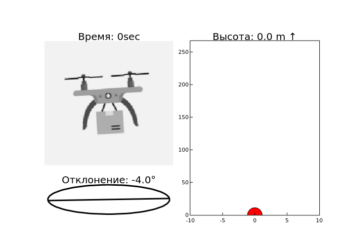
Now let's move on to the data visualization cycle itself. It can be roughly divided into three parts.
- Height display. For each time point, the height graph is plotted as a red dot.
The axis constraints are set to show the area around the current time ±10 seconds.
The chart title shows the current height value and an up/down arrow depending on whether the height is increasing or decreasing. - Pitch chart. The pitch graph shows the angle of deflection of the drone relative to the horizon.
The cosd and sind functions are used to plot the slope line.
The heading contains the pitch angle value in degrees. - Drone image rotation and visualization, the drone image is rotated by a certain angle (pitch value + 90 degrees).
The channelview function transforms the image into a view that is convenient for further processing.
A mask is used to remove black pixels.
As a result, all three graphs are assembled into a single frame that forms GIF frames.
@gif for i in 1:length(t)
    ti = t[i]
    ai = angles[i]
    hi = heights[i]

    # Height
    h_plt = scatter([ti], [hi],
        markershape=:circle, markersize=15, markercolor=:red, framestyle=:box,
        xlims = (ti-10, ti+10), ylims = (0, max_y_h),
        legend=false, grid=false,
        title="Height: $hi m $((i == 1 || heights[i] > heights[i-1]) ? "↑" : "↓")")

    # Pitch
    tang = plot([x_circle, (cosd(-ai) .* x)], [y_circle, (sind(-ai) .* x)],
        linewidth=3, color=:black, framestyle=:none,
        title="Deviation: $(ai)°")

    # The drone
    sx,sy = size(drone_img) .÷ 3;
    mini_drone = imresize( drone_img, sx, sy );
    rotated_array = channelview(Gray.(imrotate(mini_drone, π*(ai+90)/ 180, fillvalue=oneunit(eltype(mini_drone)), axes(mini_drone))));

    dron = plot(framestyle=:none, grid=false, title = "Time: $(t[i])sec")
    # Displaying the rotated image of the drone
    heatmap!(
        1:size(rotated_array, 2), 1:size(rotated_array, 1),
        permutedims(rotated_array, (2, 1)),
        colorbar=false, c=:grays
    )
    Tng_Dr = plot(dron, tang, layout = grid(2, 1, heights=[0.8, 0.2]))
    grup = plot(Tng_Dr, h_plt, layout= grid(1, 2, width = [0.75, 0.25]), legend=false)
end
Conclusion
As we can see, based on the GIF results,
we get a fairly informative representation of the data
over time. This approach can be applied
quite often, especially in cases of describing the behavior of a real physical object.