Search for key points using the ORB detector

The ORB detector is used for video stabilization, panorama creation, object detection, 3D reconstruction, camera motion estimation, image alignment, and localization for augmented reality. It is also used to recognize locations such as buildings or landmarks through a database of key points.

The theoretical part

ORB (Oriented FAST and Rotated BRIEF) is a fast keyword detector and descriptor. It combines the FAST algorithms (for detecting key points) and BRIEF (for describing them).

The FAST (Features from Accelerated Segment Test) algorithm is used to find corners in an image.
The Harris Corner Measure ** is used to select the most significant points, which reduces the number of weak key points. The orientation is calculated for each key point.
This makes the ORB invariant to image rotations.

Algorithm BRIEF (Binary Robust Independent Elementary Features) creates binary descriptors. To compare points between images, ORB uses a pairwise comparison of binary descriptors with the Hamming metric.

In this example, we will consider the classic use of the ORB detector to find key points in two images and compare them. Based on the calculated homography, the images will be aligned and combined, resulting in a panorama showing the process of combining two images into a single image.

We connect the necessary packages for working with images

import Pkg; 
Pkg.add("Images")
Pkg.add("ImageFeatures")
Pkg.add("ImageDraw")
Pkg.add("ImageProjectiveGeometry")
Pkg.add("LinearAlgebra")
Pkg.add("OffsetArrays")
Pkg.add("ImageTransformations")
Pkg.add("StaticArrays");

using Pkg, Images, ImageFeatures, ImageDraw
using ImageProjectiveGeometry
using LinearAlgebra, OffsetArrays
using ImageTransformations, StaticArrays

Uploading Images

We specify the path to the images, upload and display them:

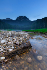
path_to_img_1 = "$(@__DIR__)/1.jpg"   
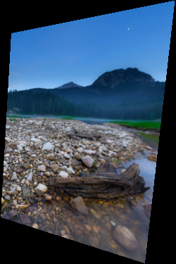
path_to_img_2 = "$(@__DIR__)/2.jpg"   

Image_1 = load(path_to_img_1)
Image_2 = load(path_to_img_2)

Application of ORB

Initializing the descriptor

orb_params = ORB(num_keypoints = 1000);

Let's define a function that uses a descriptor to search for key points in an image.

function find_features(img::AbstractArray, orb_params)
    desc, ret_features = create_descriptor(Gray.(img), orb_params)
end;

Let's define a function that searches for common key points in two images. First, the key points and descriptors for each image are calculated, then the descriptors are matched using a specified threshold.

function match_points(img1::AbstractArray, img2::AbstractArray, orb_params, threshold::Float64=0.1)
    desc_1, ret_features_1 = find_features(img1, orb_params)
    desc_2, ret_features_2 = find_features(img2, orb_params)
    matches = match_keypoints(ret_features_1, ret_features_2, desc_1, desc_2, threshold);
end;

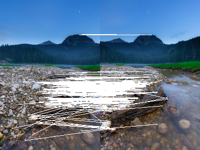
Find matching key points

matches = match_points(Image_1, Image_2, orb_params, 0.35);

Let's define a function that visualizes the relationship of key points. Function pad_display places images side by side, horizontally on the same canvas. draw_matches draws lines that connect common key points.

function pad_display(img1, img2)
    img1h = length(axes(img1, 1))
    img2h = length(axes(img2, 1))
    mx = max(img1h, img2h);

    hcat(vcat(img1, zeros(RGB{Float64},
                max(0, mx - img1h), length(axes(img1, 2)))),
        vcat(img2, zeros(RGB{Float64},
                max(0, mx - img2h), length(axes(img2, 2)))))
end

function draw_matches(img1, img2, matches)
    grid = pad_display(parent(img1), parent(img2));
    offset = CartesianIndex(0, size(img1, 2));
    for m in matches
        draw!(grid, LineSegment(m[1], m[2] + offset))
    end
    grid
end;

Let's see what we have at the exit.

draw_matches(Image_1, Image_2, matches)

Building a panorama

To calculate the homography (geometric transformation), the coordinates of the points that correspond to each other in the two images are required.

Here is from the list of matched key points matches the coordinates of the points for the two images are extracted. x1 — these are the coordinates from the first image, x2 — from the second one.

x1 = hcat([Float64[m[1].I[1], m[1].I[2]] for m in matches]...)  # 2xN
x2 = hcat([Float64[m[2].I[1], m[2].I[2]] for m in matches]...);  # 2xN

Here the RANSAC method is used to find the homography matrix H, which aligns the two groups of points as precisely as possible x1 and x2.

t = 0.01 

# Вычисление гомографии с помощью RANSAC
H, inliers = ransacfithomography(x1, x2, t);

t - this is the threshold that determines how much the points can differ after applying homography in order to be considered "correct" (inlayers).

Structure Homography to represent the homography matrix. It contains a 3x3 matrix that defines the transformation between two images.

struct Homography{T}
    m::SMatrix{3, 3, T, 9}
end

Homography(m::AbstractMatrix{T}) where {T} = Homography{T}(SMatrix{3, 3, T, 9}(m))
function (trans::Homography{M})(x::SVector{3}) where M
    out = trans.m * x
    out = out / out[end]
    SVector{2}(out[1:2])
end
function (trans::Homography{M})(x::SVector{2}) where M
    trans(SVector{3}([x[1], x[2], 1.0]))
end
function (trans::Homography{M})(x::CartesianIndex{2}) where M
    trans(SVector{3}([collect(x.I)..., 1]))
end
function (trans::Homography{M})(x::Tuple{Int, Int}) where M
    trans(CartesianIndex(x))
end
function (trans::Homography{M})(x::Array{CartesianIndex{2}, 1}) where M
    CartesianIndex{2}.([tuple(y...) for y in trunc.(Int, collect.(trans.(x)))])
end
function Base.inv(trans::Homography{M}) where M
    i = inv(trans.m)
    Homography(i ./ i[end])
end

The function is used warp to apply the homography matrix H to the image Image_1, creating a transformed image new_img.

new_img = warp(Image_1, Homography(H))

The function combines two images — the original and the transformed — into one common canvas, where a new image is added on top of the old one.

function merge_images(img1, new_img)
    # Вычисляем размеры холста
    axis1_size = max(last(axes(new_img, 1)), size(img1, 1)) - min(first(axes(new_img, 1)), 1) + 1
    axis2_size = max(last(axes(new_img, 2)), size(img1, 2)) - min(first(axes(new_img, 2)), 1) + 1

    # Создаем OffsetArray для объединённого изображения
    combined_image = OffsetArray(
        zeros(RGB{N0f8}, axis1_size, axis2_size), (
            min(0, first(axes(new_img, 1))),
            min(0, first(axes(new_img, 2)))))

    # Копируем первое изображение в общий холст
    combined_image[1:size(img1, 1), 1:size(img1, 2)] .= img1

    # Копируем второе изображение в общий холст
    for i in axes(new_img, 1)
        for j in axes(new_img, 2)
            if new_img[i, j] != colorant"black"  # Пропускаем чёрные пиксели
                combined_image[i, j] = new_img[i, j]
            end
        end
    end

    combined_image
end

merge_images (generic function with 1 method)

panorama = merge_images(Image_1, new_img)

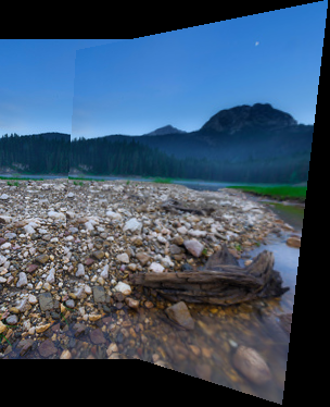
Conclusions

The example demonstrated the use of the ORB detector to automatically find key points and match them on two images. The constructed homography made it possible to align the images, and combining them made it possible to create a panorama.