Types and transformation of images

The purpose of this demonstration is to show ways to define images and the basic principles of their transformations, especially based on affine transformation.

Pkg.add(["TestImages", "ImageShow"])

using Images # Библиотека обработки изображений
using ImageShow # Библиотека отрисовки изображений
using TestImages # Библиотека тестовых изображений

Types of color spaces

Any image is just an array of pixel objects. The elements of an image are called pixels, and Julia Images treats pixels as first-class objects. For example, we have Gray pixels in shades of gray, RGB pixels of color, Lab pixels of color.

Let's start the analysis with the RGB format (an abbreviation formed from the English words red, green, blue – red, green, blue) – an additive color model that describes a way to encode colors for color reproduction using three colors, which are commonly called basic. The choice of primary colors is determined by the peculiarities of the physiology of color perception by the retina of our eye.

img_rgb = [RGB(1.0, 0.0, 0.0), RGB(0.0, 1.0, 0.0), RGB(0.0, 0.0, 1.0)]

dump(img_rgb)

Array{RGB{Float64}}((3,))
  1: RGB{Float64}
    r: Float64 1.0
    g: Float64 0.0
    b: Float64 0.0
  2: RGB{Float64}
    r: Float64 0.0
    g: Float64 1.0
    b: Float64 0.0
  3: RGB{Float64}
    r: Float64 0.0
    g: Float64 0.0
    b: Float64 1.0

Gray is a one–diagonal matrix describing images in shades of gray. By default, 8-bit color encoding is used.

img_gray = rand(Gray, 3, 3)

dump(img_gray)

Array{Gray{Float64}}((3, 3))
  1: Gray{Float64}
    val: Float64 0.20548107200013277
  2: Gray{Float64}
    val: Float64 0.7190843096024139
  3: Gray{Float64}
    val: Float64 0.7675684128936745
  4: Gray{Float64}
    val: Float64 0.4840881004197154
  5: Gray{Float64}
    val: Float64 0.21892864471268947
  6: Gray{Float64}
    val: Float64 0.5776559337062981
  7: Gray{Float64}
    val: Float64 0.855915975791712
  8: Gray{Float64}
    val: Float64 0.7152103286181891
  9: Gray{Float64}
    val: Float64 0.9976538325486705

LAB is an abbreviation for the names of two different (though similar) color spaces. The more famous and widespread is CIELAB (more precisely, CIE 1976 Lab*), the other is Hunter Lab (more precisely, Hunter L, a, b). Thus, Lab is an informal abbreviation that does not define the color space unambiguously. In Engee, when talking about the Lab space, they mean CIELAB.

img_lab = rand(Lab, 3, 3)

dump(img_gray)

Array{Gray{Float64}}((3, 3))
  1: Gray{Float64}
    val: Float64 0.20548107200013277
  2: Gray{Float64}
    val: Float64 0.7190843096024139
  3: Gray{Float64}
    val: Float64 0.7675684128936745
  4: Gray{Float64}
    val: Float64 0.4840881004197154
  5: Gray{Float64}
    val: Float64 0.21892864471268947
  6: Gray{Float64}
    val: Float64 0.5776559337062981
  7: Gray{Float64}
    val: Float64 0.855915975791712
  8: Gray{Float64}
    val: Float64 0.7152103286181891
  9: Gray{Float64}
    val: Float64 0.9976538325486705

Translation between object types

Gray.(img_rgb) # RGB => Gray

RGB.(img_gray) # Gray => RGB

RGB.(img_lab) # Lab => RGB

Image Transformation

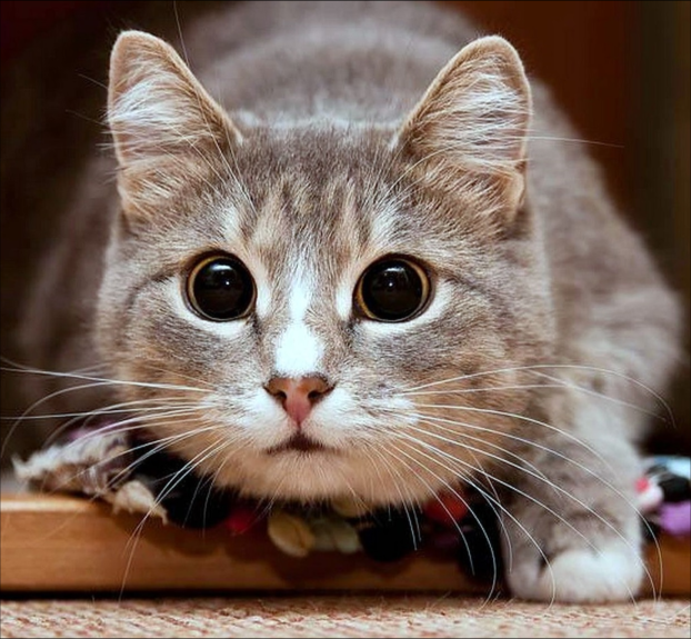
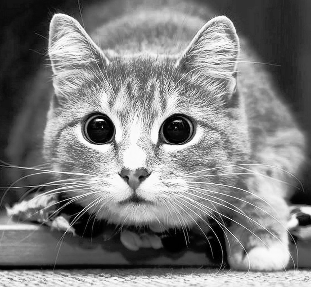
First, download the image from the .jpg file.

img = load( "$(@__DIR__)/4028965.jpg" )

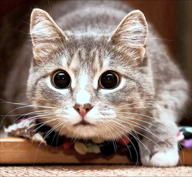
Increase the contrast of the uploaded image. Function adjust_histogram(Equalization(),...) Can handle different types of input data. The type of the returned image corresponds to the input type. For color images, the input is converted to the YIQ type, and the Y channel is aligned, after which it is combined with channels I and Q.

alg = Equalization(nbins = 256)
img_adjusted = adjust_histogram(img, alg)

Reduce the image size by 4 times relative to the source. Imresize allows you to change the size using the relationships relative to the original image, as shown in the example below, and also allows you to change the size using manual dimensionalization of the new image, for example:

imresize(img, (400, 400)).

img_small = imresize(img_adjusted, ratio=1/4)

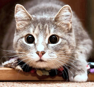
print(size(img_adjusted), " --> ", size(img_small))

(1148, 1243) --> (287, 311)

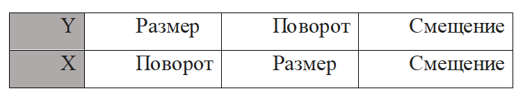
An affine transformation (from Latin affinis "touching, close, adjacent") is a mapping of a plane or space into itself, in which parallel lines turn into parallel lines, intersecting into intersecting, crossing into crossing. Basic image transformations use a grid of indexes to operate on the image. The transformation is set by the image transformation matrix according to the principle described in the picture below.

# Вспомогательная функция контроля размерностей
function C_B_V(x, max_val)
    x[x .> max_val - 1] .= max_val - 1
    x[x .< 1] .= 1
    return x
end

C_B_V (generic function with 1 method)

Next, we declare an affine image transformation function in which:

Theta is a transformation matrix;
img is the input image.;
out_size – the size of the output image;
grid – grid of pixel indexing.

function transform(theta, img, out_size)
    grid = grid = zeros(3, out_size[1]*out_size[2])
    grid[1, :] = reshape(((-1:2/(out_size[1]-1):1)*ones(1,out_size[2])), 1, size(grid,2))
    grid[2, :] = reshape((ones(out_size[1],1)*(-1:2/(out_size[2]-1):1)'), 1, size(grid,2))
    grid[3, :] = ones(Int, size(grid, 2))

    # Умножение theta на grid
    T_g = theta * grid

    # Вычисление координат x, y
    x = (T_g[1, :] .+ 1) .* (out_size[2]) / 2
    y = (T_g[2, :] .+ 1) .* (out_size[1]) / 2

    # Округление координат
    x0 = ceil.(x)
    x1 = x0 .+ 1
    y0 = ceil.(y)
    y1 = y0 .+ 1

    # Обрезание значений x0, x1, y0, y1
    x0 = C_B_V(x0, out_size[2])
    x1 = C_B_V(x1, out_size[2])
    y0 = C_B_V(y0, out_size[1])
    y1 = C_B_V(y1, out_size[1])

    # Вычисление базовых координат
    base_y0 = y0 .* out_size[1]
    base_y1 = y1 .* out_size[1]

    # Работа с изображением
    im_flat = reshape(img, :)

    # Обрабатываем координаты
    A = (x1 .- x) .* (y1 .- y) .* im_flat[Int.(base_y0 .+ x0 .+ 1)]
    B = (x1 .- x) .* (y .- y0) .* im_flat[Int.(base_y1 .+ x0 .+ 1)]
    C = (x .- x0) .* (y1 .- y) .* im_flat[Int.(base_y0 .+ x1 .+ 1)]
    D = (x .- x0) .* (y .- y0) .* im_flat[Int.(base_y1 .+ x1 .+ 1)]

    # Расчет результата
    result = reshape((A .+ B .+ C .+ D), (out_size[1], out_size[2]))
    return result
end

transform (generic function with 1 method)

First, let's apply this function to a grayscale image.

img_sg = Gray.(img_small)

As we can see from the data below, gray images have an 8-bit color depth, and its dimension is represented only by width and height.

dump(img_sg[1])

Gray{N0f8}
  val: N0f8
    i: UInt8 0x0e

size(img_sg)

(287, 311)

Let's set a transformation matrix for this image.

theta = [2 0.3 0; -0.3 2 0]

2×3 Matrix{Float64}:
  2.0  0.3  0.0
 -0.3  2.0  0.0

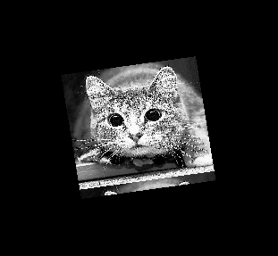
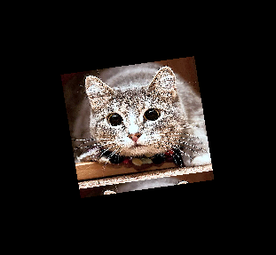
Let's apply our function to the image. As we can see, the size has been halved and the rotation has been completed.

img_transfor = transform(theta, img_sg, [size(img_sg,1),size(img_sg,2)])

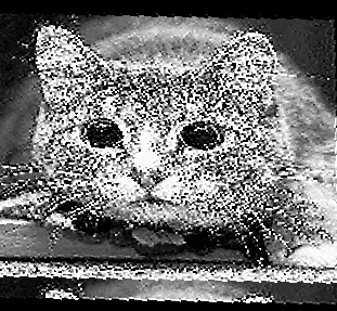
To obtain the inverse transformation, we find the inverse matrix of the transformation matrix and round it to the fourth digit.

theta_inv = hcat(inv(theta[1:2,1:2]), [-0.1;0.1])
theta_inv = round.(theta_inv.*10^4)./10^4

2×3 Matrix{Float64}:
 0.489   -0.0733  -0.1
 0.0733   0.489    0.1

img_sg_new = transform(theta_inv, img_transfor, [size(img_transfor,1),size(img_transfor,2)])

Now let's apply this function to an RGB image. First, let's convert RGB format images to a channel representation. Let's analyze the possibilities that open up to us with this image representation option.

img_CHW = channelview(img_small);
print(size(img_small), " --> ", size(img_CHW))

(287, 311) --> (3, 287, 311)

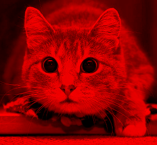
Select the red channel of the image and draw only the red channel.

RGB.(img_CHW[1,:,:], 0.0, 0.0) # red

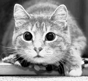
If all the channels are evenly distributed, then we will get images in shades of gray, since none of the base colors prevails over the rest.

RGB.(img_CHW[1,:,:], img_CHW[1,:,:], img_CHW[1,:,:]) # Gray

Based on the example of a channel image, we can implement an affine transformation for an RGB image by running it through our function as three separate one-dimensional matrices and combining their results.

img_CHW_new = zeros(size(img_CHW))

for i in 1:size(img_CHW,1)
   img_CHW_new[i,:,:] = transform(theta, img_CHW[i,:,:], [size(img_CHW,2),size(img_CHW,3)])
end 

RGB.(img_CHW_new[1,:,:], img_CHW_new[2,:,:], img_CHW_new[3,:,:])

Conclusion

In this demo, we have dealt with channel representations and various types of matrix representation of images, as well as analyzed some of the image processing capabilities in Engee.