Satellite image segmentation, part 2

The second example is from a series on digital image processing. In the first part we considered the problem of segmentation of a satellite image and the basic approaches to its solution. In the second part, we will look at additional methods available to a novice developer, in particular:

color segmentation
Sobel filter
The SRG algorithm

Loading necessary libraries, importing images

The next line of code should be commented out if something is missing from the application.:

Pkg.add(["Images", "ImageShow", "ImageContrastAdjustment", "ImageBinarization", "ImageMorphology", "ImageFiltering", "ImageSegmentation"])

Connecting the necessary libraries:

using Images, ImageShow, ImageContrastAdjustment, ImageBinarization, ImageMorphology, ImageFiltering, ImageSegmentation

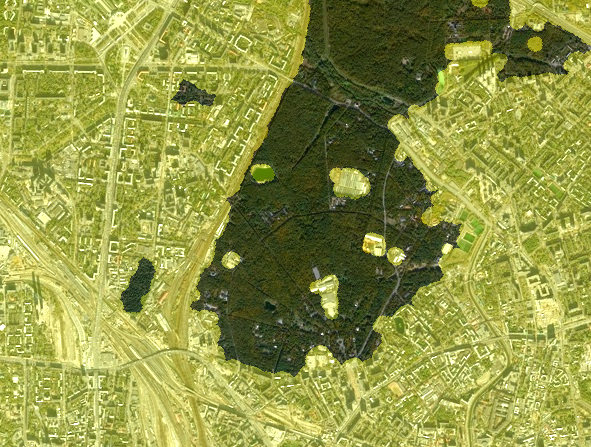
Uploading the original color image (satellite image):

I = load("$(@__DIR__)/map_small.jpg")

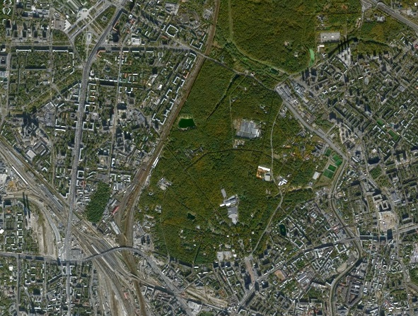
Color segmentation

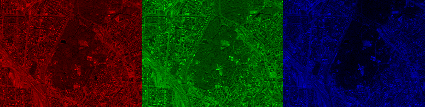
In the first part, we practically did not refer to color information, but it is obvious that the forest area is mostly green, while the city contains a lot of gray and white. This means that we can try to highlight areas that are close in color to the shade of green observed in the image. We will binarize individual image channels, and we will get access to them, as before, using the function channelview:

(h, w) = size(I);
CV = channelview(I);
[ RGB.(CV[1,:,:], 0.0, 0.0) RGB.(0.0, CV[2,:,:], 0.0) RGB.(0.0, 0.0, CV[3,:,:]) ]

A typical "green pixel" is located, presumably, in the center of the image. Let's select the "central" pixel, knowing the width and height of the image, and look at the values of its intensity in the color channels.:

midh = Int(round(h/2));
midw = Int(round(w/2));
midpixel = CV[:,midh, midw]

3-element Array{N0f8,1} with eltype N0f8:
 0.22N0f8
 0.267N0f8
 0.118N0f8

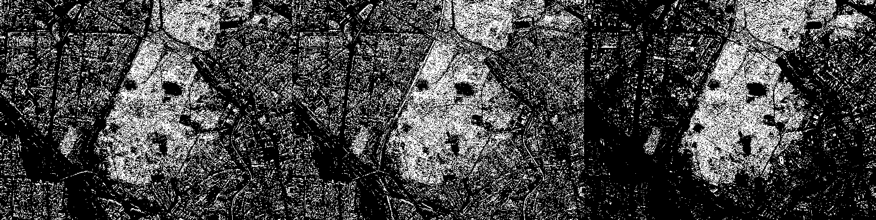
Now, using standard logical comparison operations, we binarize each of the channels. In the red channel, the logical unit will correspond to pixels with an intensity from 0.15 to 0.25, in green - from 0.2 to 0.3, and in blue - from 0.05 to 0.15.

BIN_RED = (CV[1,:,:] .> 0.15) .& (CV[1,:,:] .< 0.25) ;
BIN_GREEN = (CV[2,:,:] .> 0.2) .& (CV[2,:,:] .< 0.3);
BIN_BLUE = (CV[3,:,:] .> 0.05) .& (CV[3,:,:] .< 0.15);
simshow([BIN_RED BIN_GREEN BIN_BLUE])

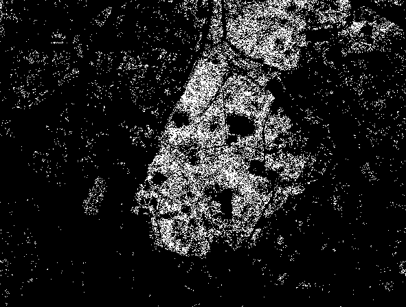
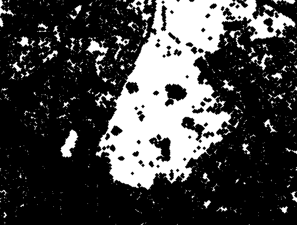
Now combine the three binary masks into one using the logical "And" operation. Now the white pixel will only be where all three conditions (ranges) are met in the original color image.:

BIN = BIN_RED .& BIN_GREEN .& BIN_BLUE;
simshow(BIN)

[Morphology] will help us make a mask out of this motley set of pixels again (https://engee.com/community/ru/catalogs/projects/morfologicheskie-operatsii-chast-1 ). This time we will take a small structural element (7x7 pixels) in the shape of a diamond.:

se = strel_diamond((7,7))

7×7 ImageMorphology.StructuringElements.SEDiamondArray{2, 2, UnitRange{Int64}, 0} with indices -3:3×-3:3:
 0  0  0  1  0  0  0
 0  0  1  1  1  0  0
 0  1  1  1  1  1  0
 1  1  1  1  1  1  1
 0  1  1  1  1  1  0
 0  0  1  1  1  0  0
 0  0  0  1  0  0  0

And let's evaluate the result of the morphological closure operation.:

closeBW = closing(BIN,se);
simshow(closeBW)

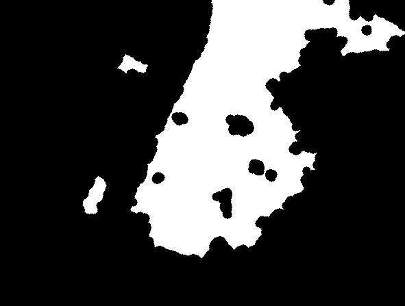
We will get the resulting mask appearance by removing small "blobs", as well as performing the closing operation again, this time to smooth out the borders of the main "large" areas of combined white pixels.:

openBW = area_opening(closeBW; min_area=500) .> 0;
se2 = Kernel.gaussian(3) .> 0.0025;
MASK_colorseg = closing(openBW,se2);
simshow(MASK_colorseg)

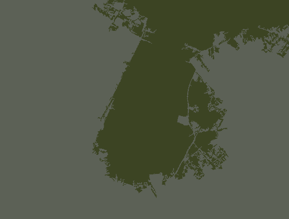
Let's apply an inverted mask to the original image in a familiar way:

sv_colorseg = StackedView(CV[1,:,:] + (.!MASK_colorseg./3), CV[2,:,:] + 
                            (.!MASK_colorseg./3), CV[3,:,:]);
view_colorseg = colorview(RGB, sv_colorseg)

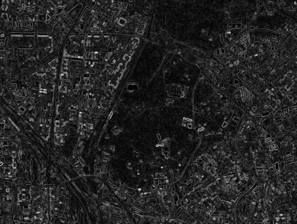
Sobel Filter

Sobel filter is an operator used in image processing to detect borders (edges of objects) based on the calculation of brightness gradients in the horizontal and vertical directions. It uses a discrete analogue of the derivative, emphasizing areas of sharp changes in pixel intensity.

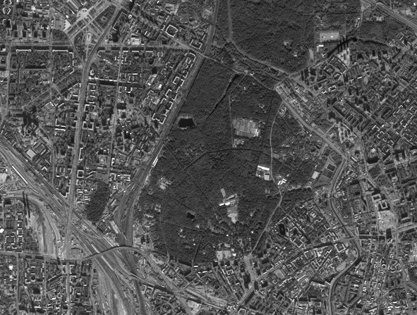
Temporarily forget about the color and we will work with the brightness map, that is, with grayscale:

imgray = Gray.(I)

The Sobel operator uses two kernels (small matrices).

On the X-axis (vertical borders):
```
[ -1  0  1 ]
[ -2  0  2 ]
[ -1  0  1 ]
```
On the Y-axis (horizontal borders):
```
[ -1 -2 -1 ]
[  0  0  0 ]
[  1  2  1 ]
```
Operating principle:
- Each core convolutes with the image, highlighting the brightness differences in its direction.
- The results are applied to the original image to obtain:
  - Gx (X-gradient),
  - Gy (Y gradient).
- The total gradient is defined as the root of the sum of the squares Gx and Gy

# Ядра Собеля для осей X и Y
sobel_x = Kernel.sobel()[1]  # Горизонтальный градиент (вертикальные границы)
sobel_y = Kernel.sobel()[2]  # Вертикальный градиент (горизонтальные границы)

# Применение свертки
gradient_x = imfilter(imgray, sobel_x)
gradient_y = imfilter(imgray, sobel_y)

# Общий градиент (объединение X и Y)
gradient_magnitude = sqrt.(gradient_x.^2 + gradient_y.^2);
imsobel = gradient_magnitude ./ maximum(gradient_magnitude)

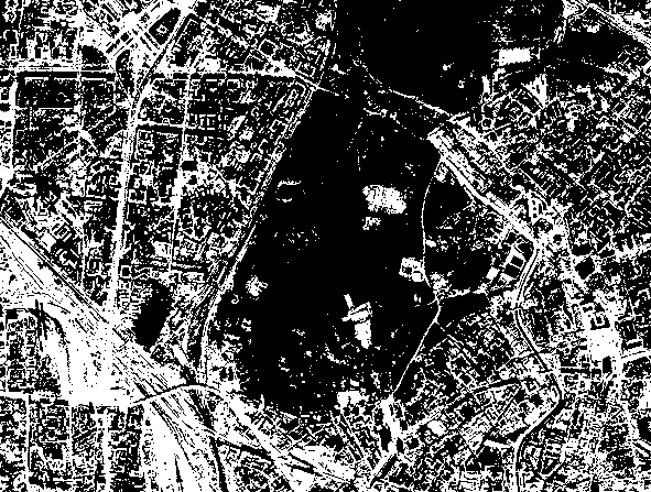
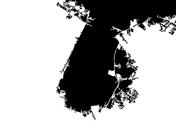
Binarize the filtering result using the Otsu method without additional arguments:

BW = binarize(imgray, Otsu());
simshow(BW)

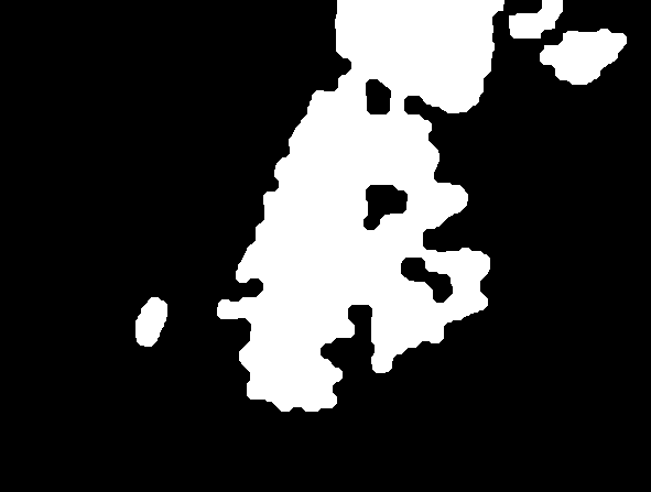
Let's add some morphological magic to get the resulting mask.:

se = Kernel.gaussian(3) .> 0.0035;
closeBW = closing(BW,se);
noobj = area_opening(closeBW; min_area=1000) .> 0;
se2 = Kernel.gaussian(5) .> 0.0027;
smooth = closing(noobj,se2);
smooth_2 = opening(smooth,se2);
MASK_sobel = area_opening(.!smooth_2; min_area=500) .> 0;
simshow(MASK_sobel)

Visualize the result:

sv_sobel = StackedView(CV[1,:,:] + (.!MASK_sobel./3), CV[2,:,:] + 
                            (.!MASK_sobel./3), CV[3,:,:]);
view_sobel = colorview(RGB, sv_sobel)

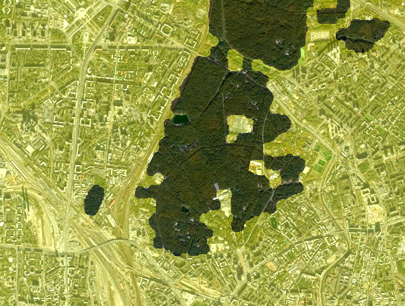
The Sobel filter was used by us as another texture filter. We took advantage of the difference in the uniformity of brightness changes in the forest and city areas.

The SRG algorithm

Seeded Region Growing (SRG) is a classic image segmentation algorithm based on the idea of combining pixels or regions into groups based on similar characteristics, starting with predefined "seed points".

Basic principles of operation:

Selection of starting points (seeds)
- The user or an automatic method selects one or more starting points (pixels) that belong to the object of interest.
Defining the similarity criterion
- The difference in intensity, color, or texture between neighboring pixels is usually used.
- For example, a pixel is added to a region if its intensity differs from the average value of the region by no more than a threshold T.
Iterative expansion of regions
- The algorithm checks the neighbors of already included pixels and adds them to the region if they meet the criterion.
- The process continues until new pixels can be added.

Let's choose the points with coordinates as the starting points. [200, 50] and [200,300]. Let's visually evaluate their colors - the success of the algorithm strongly depends on this.:

[ I[200,50] I[200,300] ]

We set the coordinates of the starting points, and we get segments (the result of segmentation) by the function seeded_region_growing by also giving her the original color image. The average color values within a segment can be found using the function segments_mean:

seeds = [(CartesianIndex(200,50),1), (CartesianIndex(200,300),2)]
segments = seeded_region_growing(I, seeds);
sm = segment_mean(segments);
[ sm[1] sm[2] ]

simshow(map(i->segment_mean(segments,i), labels_map(segments)))

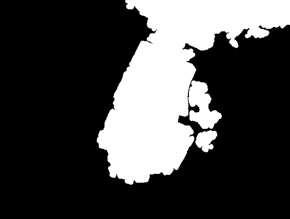
We will get a binary mask from the label matrix. We are interested in pixels with a label. 1:

lmap = labels_map(segments);
BW_smart = lmap .== 1;
simshow(BW_smart)

Well, and a bit of simple morphology:

se = Kernel.gaussian(2) .> 0.004;
closeBW = closing(BW_smart,se);
MASK_smart = area_opening(.!closeBW; min_area=500) .> 0;
simshow(MASK_smart)

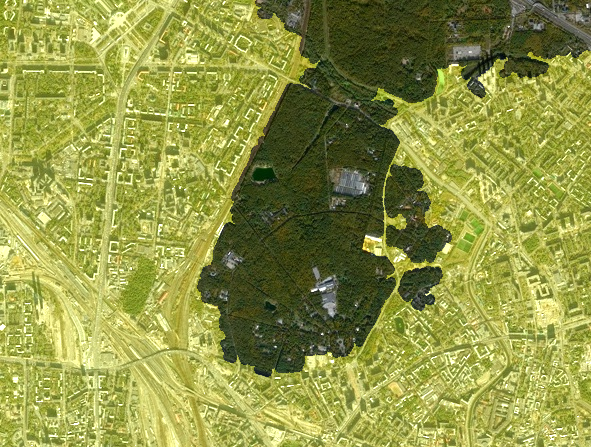
Overlay it on the original image:

sv_smart = StackedView(CV[1,:,:] + (.!MASK_smart./3), CV[2,:,:] + 
                            (.!MASK_smart./3), CV[3,:,:]);
view_smart = colorview(RGB, sv_smart)

The SRG algorithm, although it is "smart", does not apply to machine learning techniques. This is a classic algorithm in which there are no training stages and automatic feature extraction directly from the data. However, it can be combined with machine learning techniques, for example, to automatically select starting points.

Conclusion

In the second part, we examined additional image processing methods for image segmentation tasks, such as threshold color segmentation, the Sobel filter for texture analysis, and the SRG algorithm.

Next, machine learning awaits us for digital image processing tasks.