Detecting areas in the image with high temperature
In this example, we'll show you how to automatically detect objects with elevated temperatures in an image. By analyzing the image, we will identify the hot areas, as well as determine the temperature of this area. In essence, this simulates the operation of a thermal imager.
We will connect the necessary packages
import Pkg
Pkg.add("Images")
Pkg.add("ColorSchemes")
Pkg.add("ImageDraw")
Pkg.add("OpenCV")
Pkg.add("ImageMorphology")
using Images                # For working with images
using ColorSchemes          # To apply perceived color maps
using ImageDraw             # For drawing on images
using OpenCV                # To work with OpenCV
using ImageMorphology       # To perform morphological operations on images
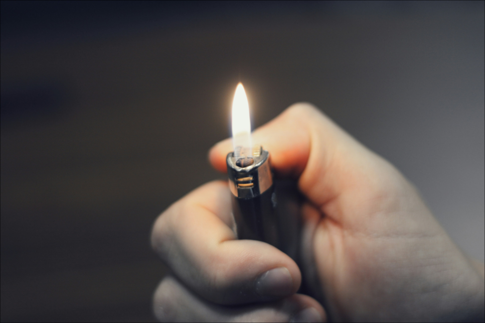
Let's upload an image with a lighter, which shows an area with elevated temperature. Using image processing techniques, we will identify an area of high temperature, as well as estimate the temperature of this area.
image = Images.load("$(@__DIR__)/lighter.jpg")
Reduce the image size for easier display:
image = imresize(image, (550, 712))

Image Conversion
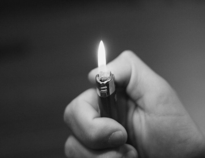
Let's convert the image to shades of gray:
image_gray = Gray.(image)
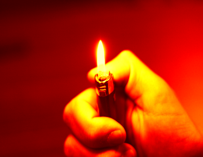
Let's upload a colormap that is used to visualize data with different intensities. On it, bright and saturated colors indicate higher values, while dark colors indicate lower values. In this example, it will be used to display areas with different temperature levels, improving the perception of temperature differences in the image.
colormap_ = ColorSchemes.hot

Let's apply the colormap to the original image using the function apply_colorscheme:
function apply_colorscheme(img, colorscheme)

    colored_img = [get(colorscheme, pixel) for pixel in img]

    return colorview(RGB, reshape(colored_img, size(img)...))
end
inferno_img = apply_colorscheme(image_gray, colormap_)
Binarization and morphological operations
Next, binarization and morphological operations will be applied to identify objects with elevated temperatures.
Binarization: This method converts an image to binary (black and white). This helps to identify only those areas that have an intensity corresponding to the range we are interested in.
Morphological operations: Morphological operations such as erosion and dilation will be applied to improve binarization results. Erosion reduces the size of objects by removing noise and small details, while dilation increases them.
Let's define the binarization threshold:
threshold = 240 / 255
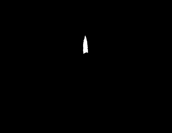
Let's perform binarization by assigning a logical unit to pixels exceeding the intensity threshold, and a logical zero to all others.:
binary_thresh = Gray.(image_gray .> threshold)

As you can see from the picture above, the resulting binary mask has an area with a flame from a lighter. However, there are noises that we will remove using morphological operations.
Define the core required for erosion and dilation:
kernel = strel_diamond((9, 9), r=2)
Let's look at the result of applying morphological operations:
BWerode = erode(binary_thresh, kernel)
BWdilate = dilate(BWerode, kernel)

As you can see from the picture above, we are left with a clearly defined area with high temperature.
Selecting a hot area into a bounding rectangle
Next, we need to limit the area of interest. To do this, we will use the methods from the OpenCV package.
We need to play around with image formats again. First, let's convert the image to RGB format.:
BWdilate = RGB.(BWdilate)
typeof(BWdilate)
Next, we will present the image in a format that OpenCV can work with.:
img_bw_raw =  collect(rawview(channelview(BWdilate)));
img_gray_CV = OpenCV.cvtColor(img_bw_raw, OpenCV.COLOR_RGB2GRAY);
Now our image is in the MAT format from OpenCV. Next, we are looking for the contours of our area.:
contours, _ = OpenCV.findContours(img_gray_CV, 1, 2)
Let's calculate the coordinates of the bounding rectangle of the area and see what they are.:
rect = OpenCV.boundingRect(contours[1])
println("Bounding box: x=$(rect.x), y=$(rect.y), width=$(rect.width), height=$(rect.height)")
Visualizing an image with a bounding rectangle
img_with_rect = draw(image, Polygon(RectanglePoints(CartesianIndex(rect.y, rect.x), CartesianIndex(rect.y + rect.height, rect.x + rect.width))), RGB{N0f8}(1.0, 0, 0.0))

Temperature detection
Next, we will determine the temperature of the selected area. The idea is to use the average pixel brightness value in this area to calculate the temperature by applying a preset calibration factor.
Let's describe a function that takes into account the calibration coefficient for the average pixel value. - convert_to_temperature:
function convert_to_temperature(pixel_avg, calibration_factor=4.6)
    return pixel_avg * calibration_factor
end;
Let's repeat the transformations for the original image in order to calculate the average value of the area, taking into account the mask. In this context, a mask is an image after morphological operations. It allows us to isolate only the area for which we want to calculate the average intensity value.
img_raw =  collect(rawview(channelview(image)));
img_gray_CV_img = OpenCV.cvtColor(img_raw, OpenCV.COLOR_RGB2GRAY);
Let's calculate the average intensity value for the region:
mean_value = OpenCV.mean(img_gray_CV_img, img_gray_CV)[1]
And convert it to temperature. The temperature values are taken on a Celsius scale:
println("Temperature of the area:", convert_to_temperature(mean_value))
Conclusions
In this example, we demonstrated the process of detecting and determining the temperature of a hot area in an image using image processing methods. We started by converting the image to a suitable format, then used binarization to highlight the areas of interest and applied morphological operations to improve the results. After that, we calculated the temperature of the selected area using a mask and a calibration coefficient to convert pixel brightness to temperature. This process eventually allows you to identify hot spots and measure their temperature, simulating the operation of a thermal imager and providing useful information for analysis.