Indexing and segmentation of images
This demo shows how to work with an indexed image using IndirectArrays, as well as the possibility of image segmentation using ImageSegmentation.
Indexation
The indexed image consists of two parts: the indexes and the pixels themselves.
The following is a "direct" representation of the image as an array.
Pkg.add(["IndirectArrays", "TestImages"])
using Images
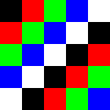
img = [
RGB(0.0, 0.0, 0.0) RGB(1.0, 0.0, 0.0) RGB(0.0, 1.0, 0.0) RGB(0.0, 0.0, 1.0) RGB(1.0, 1.0, 1.0)
RGB(1.0, 0.0, 0.0) RGB(0.0, 1.0, 0.0) RGB(0.0, 0.0, 1.0) RGB(1.0, 1.0, 1.0) RGB(0.0, 0.0, 0.0)
RGB(0.0, 1.0, 0.0) RGB(0.0, 0.0, 1.0) RGB(1.0, 1.0, 1.0) RGB(0.0, 0.0, 0.0) RGB(1.0, 0.0, 0.0)
RGB(0.0, 0.0, 1.0) RGB(1.0, 1.0, 1.0) RGB(0.0, 0.0, 0.0) RGB(1.0, 0.0, 0.0) RGB(0.0, 1.0, 0.0)
RGB(1.0, 1.0, 1.0) RGB(0.0, 0.0, 0.0) RGB(1.0, 0.0, 0.0) RGB(0.0, 1.0, 0.0) RGB(0.0, 0.0, 1.0)]
Alternatively, we could save it in indexed image format.:
indices = [1 2 3 4 5; 2 3 4 5 1; 3 4 5 1 2; 4 5 1 2 3; 5 1 2 3 4] # `i` records the pixel value `palette[i]`
palette = [RGB(0.0, 0.0, 0.0), RGB(1.0, 0.0, 0.0), RGB(0.0, 1.0, 0.0), RGB(0.0, 0.0, 1.0), RGB(1.0, 1.0, 1.0)]

palette[indices] == img
Now let's analyze the pros and cons of using IndirectArrays.
Regular indexed images may require more memory due to the storage of two separate fields. If we use unique(img), the size is close to the image's own size.
In addition, standard indexing requires two operations, so its use may be slower than direct image representation (and not amenable to SIMD vectorization).
Also, using the indexed image format with two separate arrays can be inconvenient, so IndirectArrays provides an array abstraction to combine these two parts.:
using IndirectArrays

indexed_img = IndirectArray(indices, palette)
img == indexed_img
Since an IndirectArray is just an array, common image operations are applicable to this type, for example:
new_img = imresize(indexed_img; ratio=2)
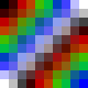
dump(indexed_img)
dump(new_img)
As we can see, after the operation on the indexed array, it was reduced to a standard array of pixels.
Segmentation
Next, we segment the image using the watershed algorithm. It is the main mathematical morphology tool for image segmentation.
using TestImages
using IndirectArrays
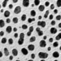
img = testimage("blobs")
img_example = zeros(Gray, 5, 5)
img_example[2:4,2:4] .=  Gray(0.6)
bw = Gray.(img) .> 0.5
bw_example = img_example .> 0.5
The feature_transform function allows us to find the transformation of the features of a binary image (bw). It finds the nearest "object" (positions where bw is in the true state) for each location in bw.
In cases where two or more objects are at the same distance, an arbitrary object is selected.
For example, the nearest true in bw_example[1,1] exists in CartesianIndex(2, 2), so it is assigned the value CartesianIndex(2, 2).
bw_transform = feature_transform(bw)
bw_transform_example = feature_transform(bw_example)
The distance transform function performs a transformation based on the specified labels.
For example, in bw_transform[1,1] there is CartesianIndex(2, 2), and D[i] for this element there will be a distance between CartesianIndex(1, 1) and CartesianIndex(2, 2), which is equal to sqrt(2).
dist = 1 .- distance_transform(bw_transform)
dist_example = 1 .- distance_transform(bw_transform_example)
the label_components function finds related components in a binary dist_trans array. You can provide a list indicating which dimensions are used to determine connectivity. For example, region = [1,3] will not be checked for the connectivity of neighbors in dimension 2. This corresponds only to the nearest neighbors, i.e. 4-connectivity in 2d and 6-connectivity in 3d matrices. The default value is region = 1:ndims(A): . The output of label is an integer array, where 0 is used for background pixels, and each individual area of connected pixels gets its own integer index.
dist_trans = dist .< 1
markers = label_components(dist_trans)
markers_example = label_components(dist_example .< 0.5)
Gray.(markers/32.0)
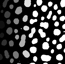
The watershed Method function segments the image using watershed transformation.
Each basin formed by watershed transformation corresponds to a segment. In the marker matrix, zero means there is no marker. If two markers have the same index, their regions will be combined into one region.
segments = watershed(dist, markers)
segments_example = watershed(dist_example , markers_example)
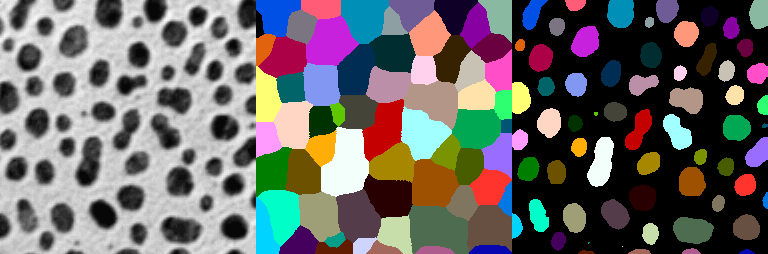
The figure below shows, from left to right, the original image, the marker areas, and the final segmented image, which break down the image segments by color.
labels = labels_map(segments)
colored_labels = IndirectArray(labels, distinguishable_colors(maximum(labels)))
masked_colored_labels = colored_labels .* (1 .- bw)
mosaic(img, colored_labels, masked_colored_labels; nrow=1)
Conclusion
In this demo, we showed how to use image indexing to segment individual image areas. These methods can be useful in extracting areas of interest from the original image.