Segmentation of a satellite image, part 1
This is the first example from a series of scripts
describing typical digital
image processing tasks. In the first part, we will get acquainted with
the basic approaches and algorithms of image processing
for the task of segmentation of a satellite image.
Segmentation is the mapping
of image pixels to different classes.
In the simplest case, you can separate
objects in the conditional "foreground"
from objects in the conditional "background".
In this case, the result of segmentation
can be a binary mask matrix of the same
size as the original image, where
elements 1 correspond
to the objects of interest, and elements 0 correspond to the background.
Topics covered:
- Import and visualization of digital images
- linear and nonlinear filtering
- morphological operations
- Development of custom functions
Download necessary libraries, import data
The next line of code should
be commented out if something is missing from the application.:
# Pkg.add(["Images", "ImageShow", "ImageContrastAdjustment", "ImageBinarization", "ImageMorphology"])
Connecting downloaded libraries:
using Images, ImageShow, ImageContrastAdjustment, ImageBinarization, ImageMorphology
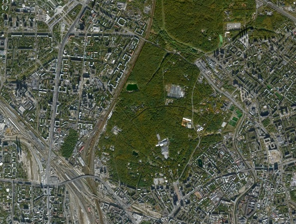
Loading and visualizing the original
color image with the function load.
The processed image
is a satellite image
of a small area of the city map,
which contains both
areas of development and a forest belt.
Our task is to try to separate
the forest from the city.
I = load("$(@__DIR__)/map_small.jpg") # uploading the original color image
Preprocessing
As a rule, preprocessing tasks
include image analysis to highlight
the characteristic features of objects (their differences from the background),
contrast and/or brightness changes,
filtering to remove noise or smooth texture,
and so on.
Let's consider which of the preprocessing algorithms
are suitable in our case. Given that the image
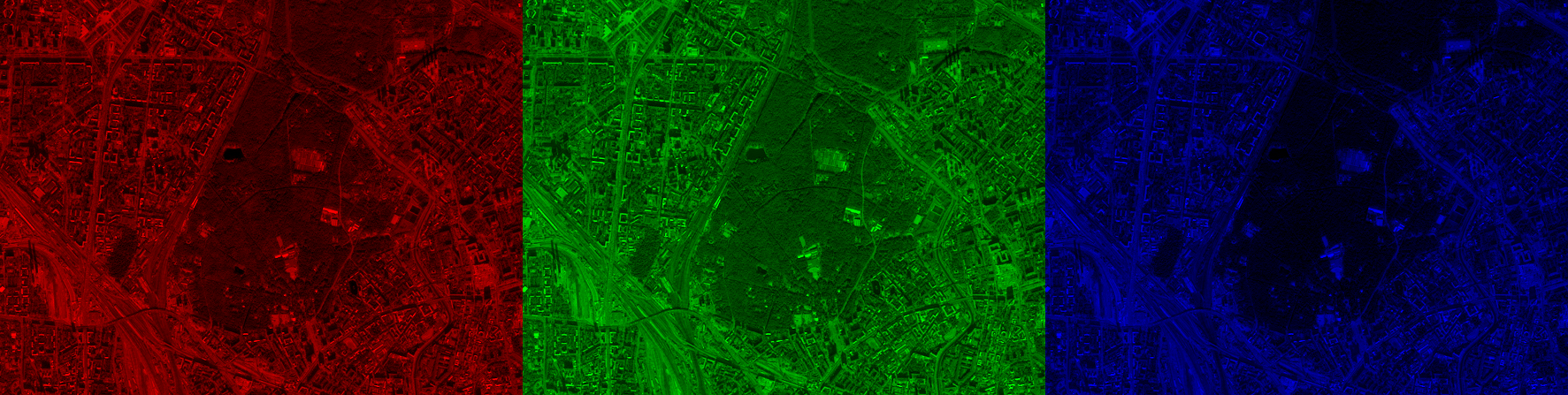
is in color, you can try to consider separate
channels (red, green and blue). To do this
, use the function channelview:
h = size(I, 1);         # image height, pixels
CV = channelview(I);    # decomposing an image into channels
[ RGB.(CV[1,:,:], 0.0, 0.0) RGB.(0.0, CV[2,:,:], 0.0) RGB.(0.0, 0.0, CV[3,:,:]) ]
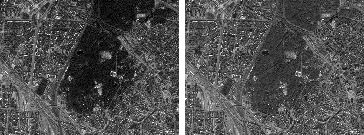
In order to get a binary mask,
we need to work with a
grayscale image (the so-called intensity matrix).
We can convert a color image to
the intensity matrix by the function Gray or
consider one of the channels. As we can see,
in the blue channel, the forest area in the image
differs more in intensity from
the city area. And the task of segmentation is to separate
the brighter areas of pixels from the darker ones.
[RGB.(CV[3,:,:]) simshow(ones(h,20)) Gray.(I)]
Now let's use a linear smoothing filter
to even out the intensity of closely spaced
pixels in the blue channel. Let's compare two linear
filters - a Gaussian filter with
a sliding window measuring 9 by 9 pixels, as well
as a simple averaging filter with a window measuring 7 by 7.
Let's apply them to the matrix BLUE using the function
imfilter to which we will transfer different kernels.
BLUE = CV[3,:,:];                                       # RGB blue channel intensity
gaussIMG = imfilter(BLUE, Kernel.gaussian(2));          # linear Gauss filter
kernel_average = ones(7,7) .* 1/(7^2);                  # the kernel of the arithmetic mean
avgIMG = imfilter(BLUE, kernel_average);                # linear average filter
[simshow(gaussIMG) simshow(ones(h,20)) simshow(avgIMG)]
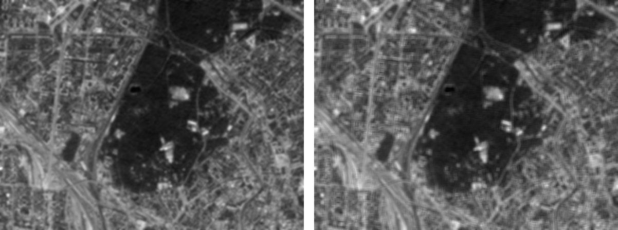
With the selected parameters of the cores used,
the result is not fundamentally different and we are quite
satisfied. As the main image for
further operations, we take the result of a simple
averaging filter, the matrix avgIMG.
Binarization
Binarization is the process of obtaining a matrix
containing binary values, i.e. 1 or 0.
In the image, this corresponds to the white and
black pixels. In segmentation, white pixels
will correspond
to one of the classes, and black pixels to the other.
Let's compare two binarization methods - the Otsu method,
available through the function binarize, and a simple
comparison of intensity to a threshold value.
binOTSU = binarize(avgIMG, Otsu());         # binarization by the Otsu method
binTHRESH = avgIMG .> 0.25;                 # binarization at a threshold of 0.25
BW_AVG = binTHRESH;
[ simshow(binOTSU) simshow(zeros(h,20)) simshow(binTHRESH) ]

The results are also almost identical,
and we will continue with the binary image after
a simple comparison with the threshold.
Despite the fact that we got a binary
matrix, a mask, there is a lot of noise on it: the areas
have gaps, "slits", there are many
small objects. To make the mask
smoother and noise-free, we will use
binary morphology algorithms.
Morphological operations
Morphological operations can be performed
on both binary images and
intensity matrices. But to understand the basic
algorithms, we will limit ourselves to binary
morphology.
The basic algorithms, such as dilation,
opening, closing, or erosion, use
special kernels - structural elements.
Parameterized functions are available to us to create
typical "rhombus" or "square" type structural elements,
however, we are interested in creating a round structural
element. Therefore, we binarize the two-dimensional
Gaussian distribution with a threshold of 0.0025.
kernel_d = strel_diamond((13, 13), r=6);       # The "rhombus" structural element
kernel_b = strel_box((13, 13), r=4);           # The "square" structural element
se = Kernel.gaussian(3) .> 0.0025;             # the "custom" structural element
[ simshow(kernel_d) simshow(zeros(13,13)) simshow(kernel_b) simshow(zeros(13,13)) simshow(se) ]

Now let's perform the morphological closure operation
with the function closing
with a custom structural element. This will allow
you to "close" small holes and gaps between white
pixels, as well as smooth out the shape of objects (blobs).
We consider objects to be "combined" areas of white
pixels surrounded by black pixels, or the border
of the image.
After the closing operation, we will use
the function area_open and we will delete objects whose size
does not exceed 500 pixels.
closeBW = closing(BW_AVG,se);                           # morphological closure
openBW = area_opening(closeBW; min_area=500) .> 0;      # deleting "small" objects
[ simshow(closeBW) simshow(zeros(h,20)) simshow(openBW) ]

Now we invert our binary mask
and remove objects less than 5000 pixels in size.
We will also smooth out the inverted mask
with the closing operation.:
fillBW = imfill(.!openBW, (0,5000));            # deleting "large" objects
MASK_AVG = closing(fillBW,se);                  # morphological closure (smoothing)
[ simshow(fillBW) simshow(ones(h,20)) simshow(MASK_AVG) ]

Segmentation result
We want to make sure that the resulting
binary mask segments the original image.
To do this, the images need to be combined.
For our chosen visualization, we will add 30%
of the intensity of the binary mask to the red and
green channels of the original color image.
Thus, we get a translucent
yellow mask.:
sv1_AVG = StackedView(CV[1,:,:] + (MASK_AVG./3), CV[2,:,:] +
                            (MASK_AVG./3), CV[3,:,:]);          # applying the "yellow mask"
forest_AVG = colorview(RGB, sv1_AVG);
sv2_AVG = StackedView(CV[1,:,:] + (.!MASK_AVG./3), CV[2,:,:] +
                            (.!MASK_AVG./3), CV[3,:,:]);        # applying the "yellow mask"
city_AVG = colorview(RGB, sv2_AVG);
[ forest_AVG simshow(ones(h,20)) city_AVG ]
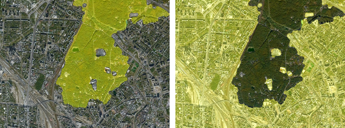
Visually, we can assess the result as good.
We are witnessing the successful allocation of the forest area.
The algorithm is not universal, because
Many
algorithm parameters were matched to similar
test images. However, the purpose of the example is
to demonstrate the process of developing prototypes
of the algorithms of the Central Research Institute.
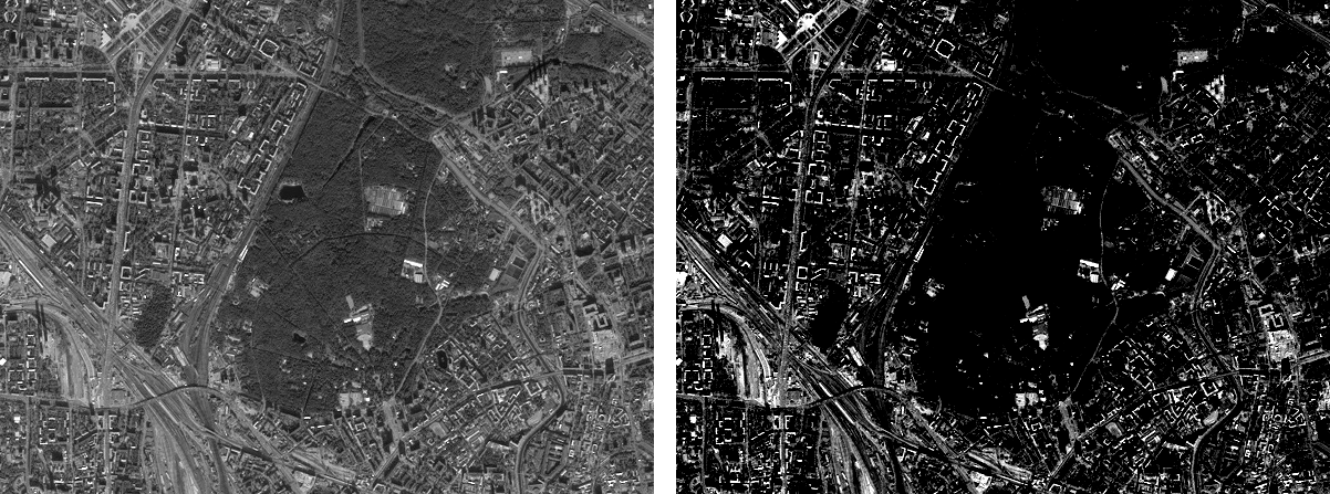
Nonlinear filtering
Let's consider another approach to
image preprocessing. In this case, we will use
the stretching of the histogram of the image
in grayscale, as well as a nonlinear
texture filter.
To begin with, let's apply the function to a monochrome image
adjust_histogram with the method
LinearStretching. We got a very
contrasting image with a large number of
bright and dark pixels.
IMG = adjust_histogram(Gray.(I), LinearStretching(dst_minval = -1, dst_maxval = 1.8));
[ Gray.(I) simshow(ones(h,20)) IMG ]
Now let's use the so-called range filter.
This is a nonlinear filter that
determines the difference between the maximum and minimum intensity of the array inside the sliding core
.
To do this, let's write a simple custom function
range, which is based on the built-in function
extrema, which returns two values.
function range(array)                           # nonlinear filtering function
    (minval, maxval) = extrema(array);          # min. and max. array values
    return maxval - minval;                     # range (max. - min.)
end
Let's apply a custom function to a window sliding
across the image using the function mapwindow.
The result of nonlinear filtering is binarized by the Otsu method.
rangeIMG = mapwindow(range, IMG, (7,7));        # the `range` function in the 7x7 window
BW_RNG = binarize(rangeIMG, Otsu());            # binarization by the Otsu method
[ rangeIMG simshow(zeros(h,20)) BW_RNG ]
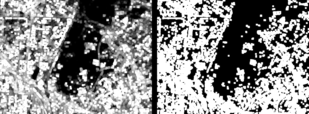
In the area of urban development
, the pixel intensity varies more strongly and
spatially more often than in the forest belt area.
Therefore, texture filters can be used to
separate areas in images whose average intensity
varies slightly after standard
linear filters.
Custom Morphology function
Let's combine the operations following binarization
into one function. myMorphology and apply it
to a binary image.:
function myMorphology(BW)
    se = Kernel.gaussian(3) .> 0.0025;
    closeBW = closing(BW,se);
    openBW = area_opening(closeBW; min_area=500) .> 0;
    fillBW = imfill(.!openBW, (0,5000));
    MASK = closing(fillBW,se);
    return MASK
end
Visualize the resulting mask:
MASK_RNG = myMorphology(BW_RNG);
sv1_RNG = StackedView(CV[1,:,:] + (MASK_RNG./3), CV[2,:,:] +
                            (MASK_RNG./3), CV[3,:,:]);
forest_RNG = colorview(RGB, sv1_RNG);
sv2_RNG = StackedView(CV[1,:,:] + (.!MASK_RNG./3), CV[2,:,:] +
                            (.!MASK_RNG./3), CV[3,:,:]);
city_RNG = colorview(RGB, sv2_RNG);
[ forest_RNG simshow(ones(h,20)) city_RNG ]
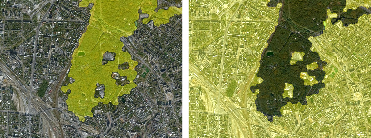
Try to compare the results of linear
and nonlinear filtering programmatically.
Custom segmentation function
Finally, we will assemble all the sequential
algorithms of preprocessing, nonlinear filtering
and morphology into another function. mySegRange,
which accepts a color image as input:
function mySegRange(I)
    CV = channelview(I);
    IMG = adjust_histogram(Gray.(I), LinearStretching(dst_minval = -1, dst_maxval = 1.8));
    rangeIMG = mapwindow(range, IMG, (7,7));
    BW_RNG = binarize(rangeIMG, Otsu());
    MASK_RNG = myMorphology(BW_RNG);
    return MASK_RNG
end
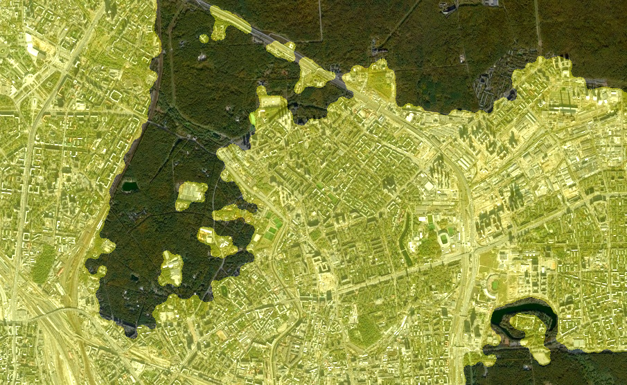
And apply it to a larger snapshot of the area.:
I2 = load("$(@__DIR__)/map_big.jpg");
CV2 = channelview(I2);

myMASK = mySegRange(I2);

sview = StackedView(CV2[1,:,:] + (.!myMASK./3), CV2[2,:,:] + (.!myMASK./3), CV2[3,:,:]);
colorview(RGB, sview)
The practical meaning of such operations is the ability
to perform analysis and calculations on selected
objects in automatic mode.
Knowing the linear dimensions of a pixel on the map in meters, you can,
for example,
determine the area of objects on the map.
In our case, we can calculate the area (in km^2)
occupied by the forest belt, urban development, as well
as the percentage of forest to the total area
of the site under consideration.:
pixsquare = (800/74)^2;                   # the area of one pixel of the map raster (km^2)
forest_area_km2 = round((sum(myMASK) * pixsquare) / 1e6, sigdigits = 4) # forest area
city_area_km2 = round((sum(.!myMASK) * pixsquare) / 1e6, sigdigits = 4) # city square
forest_percentage = round(100*sum(myMASK)/length(I2), sigdigits = 4) # percentage of forest
Conclusion
Using the example of satellite image processing, we got acquainted
with various methods of image preprocessing,
binarization, and morphological operations for
segmentation tasks, and also learned how to quickly develop
custom digital image processing functions.