Eliminating noise in an image using reverse convolution

Let's apply algorithms to eliminate noise and blurring in the image using the library Deconvolution.

Task description

Deconvolution or reverse convolution (deconv) is an operation that is the reverse of convolution, which allows you to obtain the original signal (or restore the image) with a known or estimated filter model. In our scenario, when we improve image quality, by filter we mean the description of the process that has interfered with our image (blur, smudge, noise, etc.).

The characteristics of this process are usually difficult to know in advance, and the reverse convolution operation itself is very sensitive to errors in the filter coefficients. This should be taken into account when creating a procedure for evaluating the parameters of the filter model.

Here are the libraries that we will need:

Pkg.add( ["Images", "TestImages", "Deconvolution", "FFTW", "ZernikePolynomials"] )

Wiener's inverse convolution

Let's upload the experimental image and add noise to it. Replacing the function textimage("image") on load("image.png") you can open any image from the disc.

using Images, TestImages, Deconvolution, FFTW

img = channelview(testimage("cameraman"))

# Создадим размывающий фильтр в частотной области
x = hcat(ntuple(x -> collect((1:512) .- 257), 512)...)
k = 0.001
blurring_ft = @. exp(-k*(x ^ 2 + x ^ 2)^(5//6))

# а еще у нас будет аддитивный шум
noise = rand(Float64, size(img))

# Преобразование Фурье позволяет получить картинку с шумом
blurred_img_ft = fftshift(blurring_ft) .* fft(img) .+ fft(noise)

# Преобразуем изображение из частотной в пространственную область (восстановим из спектра)
blurred_img = real(ifft(blurred_img_ft))

# Также получим фильтр в пространственной области
blurring = ifft(fftshift(blurring_ft));

Now let's perform the reverse convolution operation and output three images glued into one:

the original image,
invention with added noise,
filtered image.

polished = wiener(blurred_img, img, noise, blurring)

[ Gray.( img ) Gray.(blurred_img) Gray.( polished ) ]

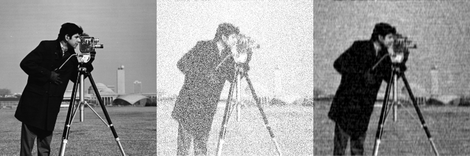
We see the original image, then the blurred image with added noise, and the restored distortion.

Wiener's inverse convolution also works when we do not have the original image and the filter model (that is, in the usual realistic scenario). The reverse convolution can be performed with only a rough understanding of the power spectra of the original signal and filter.

img2 = channelview( testimage("livingroom") ) # Загрузим другое изображение
noise2 = rand(Float64, size(img)) # Другая модель шума с 

# Уберем шум с пролого изображения при помощи обратной свертки
polished2 = wiener( blurred_img, img2, noise2, blurring );

[ Gray.( img2 ) Gray.( polished2 ) ]

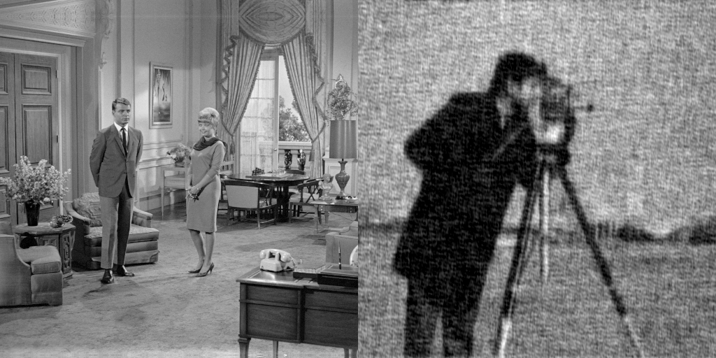
The image on the left gave the algorithm an idea of what the spectrum of the cleared image should look like. And since we didn't model the blur when creating the filter noise2 the result was less clear.

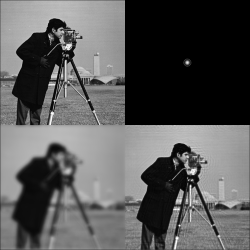
The reverse convolution of Richardson-Lucy

As a second example, we use the function lucy, which implements the Richardson-Lucy inverse convolution method on an image that has been blurred using an aberration model.

using Images, TestImages, Deconvolution, FFTW, ZernikePolynomials

img = channelview( testimage("cameraman") )

# Модели аберрации линзы
blurring = evaluatezernike( LinRange(-16,16,512), OSA.([12, 4, 0]), [1.0, -1.0, 2.0] )
blurring = fftshift(blurring)
blurring = blurring ./ sum(blurring)

blurred_img = fft(img) .* fft(blurring) |> ifft |> real

@time restored_img = lucy(blurred_img, blurring, iterations=1000)

[ Gray.(img)  Gray.( fftshift(blurring .* 255));
  Gray.(blurred_img) Gray.(restored_img) ]

 55.638180 seconds (36.03 k allocations: 35.187 GiB, 0.79% gc time)

Conclusion

We have successfully tested a couple of image recovery algorithms and got good results.