Video processing — object boundary analysis
In this paper, a method for constructing energy maps for video sequences is considered.
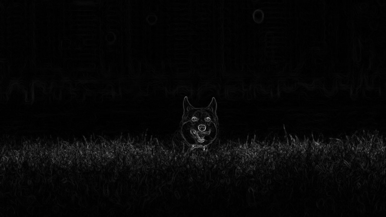
The energy map, calculated as the Euclidean norm of brightness gradients, is a key component in computer vision algorithms such as seam carving and contour highlighting.
We have presented an implementation in the Julia language, which includes a debugging stage on a single static frame and subsequent optimized processing of the video data stream.
To ensure performance, memory preallocation techniques and operation vectorization are used. The result of the work is a script that generates visual animation in GIF format, which demonstrates the dynamic change of energy maps over time. First, let's look at the original video.
include("player.jl")
media_player("input.mp4", mode="video")
Now let's move on to implementing a simple processing example. The purpose of this script is to read the first frame from a video file. input.mp4, convert it to a black-and-white image, calculate an energy map, visualize the result and save it to a file, as well as output basic statistics, then analyze the script point by point.
This script is research and debugging, it is designed to verify the correctness of the algorithm on a single static frame before using it in more complex and resource-intensive tasks.
1. Import necessary libraries
Images.jl: The main package for working with images (loading, saving, basic pixel operations).ImageFiltering.jl: Provides features for image filtering such asimfilter, which is used to apply convolution kernels (in this case, the Sobel operator).VideoIO.jl: A package for reading and writing video files. It is used here to open videos and extract frames.
Pkg.add(["Images", "ImageFiltering", "VideoIO"])
using Images, ImageFiltering, VideoIO
2. RGB to Grayscale conversion function, this function uses standard brightness perception coefficients by the human eye, the purpose of the function is to convert one pixel of a color image (RGB) into its brightness value (grayscale).
pixel::AbstractRGB: Function argument. Type annotation::AbstractRGBspecifies that the function expects an object representing an RGB pixel as input.::Float64: The annotation of the return type indicates that the function will return a double-precision floating-point number.- Formula (
0.299 * R + 0.587 * G + 0.114 * B): These are the standard coefficients (ITU-R BT.601) used to convert a color image to grayscale. They take into account the different sensitivity of the human eye to different colors (green is perceived as the brightest, blue as the darkest). red(pixel),green(pixel),blue(pixel): Functions from the packageImages.jl, which extract the corresponding color channel from a pixel. The returned values are usually normalized to a range of[0, 1].
function calculate_brightness(pixel::AbstractRGB)::Float64
    return 0.299 * red(pixel) + 0.587 * green(pixel) + 0.114 * blue(pixel)
end
3. The energy map calculation function takes a color image and returns its energy map.
image::AbstractMatrix{<:AbstractRGB}The input image is represented as a two—dimensional array (matrix), where each element is an RGB pixel.- The key argument
sobel_kernel: Allows you to transfer custom convolution kernels. By default, Sobel operator kernels are used.(Kernel.sobel()[1], Kernel.sobel()[2]), which are returned by the functionKernel.sobel()fromImageFiltering.jl. ::Matrix{Float64}: The function returns a matrix of numbersFloat64, which is the energy map.- Formula:
energy = sqrt(Gx² + Gy²). This calculates the magnitude (modulus) of the gradient vector at each point.- A high energy value means a sudden change in brightness (object edge, texture).
- A low energy value means a smooth transition or a homogeneous area (sky, blurred background).
function calculate_energy(image::AbstractMatrix{<:AbstractRGB};
    sobel_kernel::Tuple=(Kernel.sobel()[1], Kernel.sobel()[2]))::Matrix{Float64}
# Converting to grayscale
gray_image = calculate_brightness.(image)
# Calculating gradients along the X and Y axes
gradient_x = imfilter(gray_image, sobel_kernel[1])
gradient_y = imfilter(gray_image, sobel_kernel[2])
# We calculate the energy as the Euclidean norm of the gradients
energy_map = sqrt.(gradient_x.^2 + gradient_y.^2)
return energy_map
end
4. Main part of the script: Video processing
VideoIO.openvideo("input.mp4")Opens the video file for reading.read(video): Reads the next frame from the video. Since the video has just been opened, this will be the first frame.close(video)It is important to close the video file immediately after reading the necessary data to free up resources.size(frame)Outputs the dimension of the frame matrix (for example,(720, 1280)— height and width in pixels).eltype(frame): Outputs the type of matrix elements (for example,RGB{N0f8}— RGB pixel, where each channel is represented by an 8-bit unsigned normalized number[0, 1]).
println("Video reading...")
println()
video = VideoIO.openvideo("input.mp4")
frame = read(video)
close(video)
println("Frame size: ", size(frame))
println("Data type: ", eltype(frame))
5. Calculation, normalization and conservation of the energy map.
@time: A macro that measures the execution time and the amount of allocated memory for the expression calculate_energy(frame). Useful for profiling.
println("Calculating the energy map...")
@time energy_result = calculate_energy(frame)
Normalization: Source energy map energy_result it has an arbitrary range of values. To save it correctly as an image (where the pixel values should be in the range [0, 1] for Float or [0, 255] for integers), we divide each element by the maximum value in the matrix. This scales all the values into an interval [0.0, 1.0].
energy_normalized = energy_result ./ maximum(energy_result)
save: Function from the package Images.jl to save the image. By default, it understands that the matrix of floating-point numbers is in the range [0,1] it must be saved as a grayscale image.
save("first_frame_energy_improved.png", energy_normalized)
load...display Downloads the newly saved image and displays it directly in the runtime environment to view the result.
display(load("first_frame_energy_improved.png"))
6. Statistics output
maximum/minimum Shows the actual range of values on the energy map before normalization. It helps to understand the dynamic range of the data. The minimum value close to zero (8.13e-17), is expected for homogeneous regions, and the maximum (~0.26) indicates the strength of the most contrasting borders.
println("Maximum energy value: ", maximum(energy_result))
println("Minimum energy value: ", minimum(energy_result))
Next, let's look at the modified algorithm, its code is an optimized version for batch video processing, radically different from the previous script, which analyzed only one frame. The key difference lies in the transition from a single calculation to streaming processing of multiple frames with the creation of animated visualization.
The principle of operation is based on pre-allocation of memory for buffers (gray_buffer, energy_buffer, frame_matrix), which eliminates the re-creation of arrays for each frame and significantly speeds up calculations. Function calculate_energy_fast! uses vectorized operations (@.) and single precision types (Float32) to optimize performance, and also works with externally transferred buffers, avoiding costly memory allocation.
The main loop sequentially reads the frames, calculates an energy map for each, creates a heatmap with preset visualization settings, and adds the frame to the animation. As a result, a GIF animation is formed that clearly demonstrates the dynamics of changes in energy maps over time for the first 40 frames of the video, which provides a qualitatively new level of analysis compared to a static image of a single frame.
using Images, ImageFiltering, VideoIO

function calculate_energy_fast!(output::Matrix{Float32}, image::AbstractMatrix{<:AbstractRGB},
                               gray_buffer::Matrix{Float32}, sobel_x, sobel_y)
    @. gray_buffer = 0.299f0 * red.(image) + 0.587f0 * green.(image) + 0.114f0 * blue.(image)
    gradient_x = imfilter(gray_buffer, sobel_x)
    gradient_y = imfilter(gray_buffer, sobel_y)
    @. output = sqrt(gradient_x^2 + gradient_y^2)
    return output
end

function process_video_energy()
    video = VideoIO.openvideo("input.mp4")
    frame_count = counttotalframes(video)
    anim = Animation()
    sobel_x, sobel_y = Kernel.sobel()
    first_frame = read(video)
    seek(video, 1)
    frame_matrix = collect(first_frame)
    h, w = size(frame_matrix)
    gray_buffer = Matrix{Float32}(undef, h, w)
    energy_buffer = Matrix{Float32}(undef, h, w)
    heatmap_settings = (color = :viridis, aspect_ratio = :equal, axis = false, colorbar = false, size = (600, 400), dpi = 80)
    total_frames = min(40, frame_count)
    println("Creating a GIF...")
    gif_output = "energy_animation.gif"
    for i in 1:total_frames
        frame = read(video)
        copyto!(frame_matrix, frame)
        calculate_energy_fast!(energy_buffer, frame_matrix, gray_buffer, sobel_x, sobel_y)
        plt = heatmap(reverse(energy_buffer); heatmap_settings...)
        Plots.frame(anim)
        if i % 20 == 0
            println("Processed $i of $total_frames frames")
        end
    end
    close(video)
    display(gif(anim, gif_output, fps=10))
    println("Animation saved as '$gif_output'")
end
@time process_video_energy()
Conclusion
These examples are a comprehensive tutorial on modern image and video processing, revealing several key aspects of programming in a scientific environment.
This example examines issues such as:
- Debugging methodology: Start by verifying the algorithm on small data before scaling
- Optimization of calculations: Using preallocation, correct data types (Float32), vectorization
- Working with memory: Avoiding unnecessary memory allocations in cycles
- Creating reproducible results: Export and visualization of data at all stages of processing
These examples demonstrate the full cycle of scientific programming - from research to optimized code, which makes them valuable material for mastering modern methods of multimedia data processing.