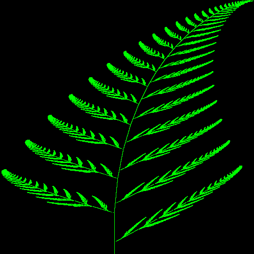
The Barnsley Fern

The implementation of the well-known fractal algorithm "Barnsley's Fern", which generates an image of a fern using a system of iterated functions, is considered.

Introduction

The Barnsley Fern algorithm is an example of using the Iterated Function System (IFS) to generate fractals. It was proposed by mathematician Michael Barnsley and allows you to create a realistic image of a fern leaf by applying simple affine transformations with a certain probability.

A fractal is constructed by repeatedly applying random affine transformations to a point on the plane. Each of the four transformations corresponds to a specific part of the plant (stem, left branch, right branch, and tip), and the probabilities of choosing these transformations determine the characteristic appearance of the fern.

This algorithm is widely used as an educational example in fractal theory and computer graphics due to its clarity and mathematical beauty.

# Installing the required package
import Pkg; Pkg.add("Images")

using Images

The main part

Defining the structure `BarnsleyFern`

mutable struct defines a mutable data structure in which all parameters and the current state of our fractal will be stored.

mutable struct BarnsleyFern
    # the size of the image in width and height in pixels
    width::Int
    height::Int
    # the color that the fern will be drawn with
    color::RGB
    # the current coordinates of the point are x and y
    x::Float64
    y::Float64
    # two-dimensional array (matrix) of image pixels
    fern::Matrix{RGB}

    # Structure constructor. Called when creating a new BarnsleyFern() object
    function BarnsleyFern(width, height, color = RGB(0.0, 1.0, 0.0), bgcolor = RGB(0.0, 0.0, 0.0))
        # Creating an empty image with the size width by height,
        # filling it with the background color bgcolor
        img = [bgcolor for x in 1:width, y in 1:height]
        
        # Calculating the initial coordinates of the center point in pixels:
        # cx is calculated taking into account the range of x values from -2.182 to 2.6558 (approximately 4.8378)
        cx = Int(floor(2.182 * (width - 1) / 4.8378) + 1)
        # cy is calculated taking into account the range of y values from 0 to 9.9983
        cy = Int(floor(9.9983 * (height - 1) / 9.9983) + 1)
        
        # Setting the first pixel at the starting point
        img[cx, cy] = color
        
        # Creating a new instance of the BarnsleyFern structure
        # with the specified parameters and initialized image matrix
        return new(width, height, color, 0.0, 0.0, img)
    end
end

Structure BarnsleyFern It contains information about the size of the image, the current position of the point, the color of the rendering, and the pixel matrix itself. The constructor creates a black background rectangle and sets the starting point of the fern growth in the lower central area of the drawing area.

Defining a point transformation

A function that performs one iteration of the algorithm: selects one of the four affine transformations and applies it to the current coordinates of the point (f.x, f.y), then converts the new real coordinates to discrete pixel coordinates and fills in the corresponding pixel in the image.

function transform(f::BarnsleyFern)
    # Generating a random number from 0 to 99 (inclusive)
    r = rand(0:99)
    
    # Depending on the value of r, one of 4 affine transformations is selected.:
    # The probabilities are chosen so that you get a realistic view of the fern.:
    # 1% — vertical compression (trunk)
    # 85% — large leaves on top (main transformation)
    # 7% — small leaves on the left
    # 7% — small leaves on the right
    
    if r < 1
        # Turning a point into the root of the trunk
        f.x = 0.0
        f.y = 0.16 * f.y
    elseif r < 86
        # Main transformation: formation of the main mass of foliage
        f.x = 0.85 * f.x + 0.04 * f.y
        f.y = -0.04 * f.x + 0.85 * f.y + 1.6
    elseif r < 93
        # Formation of the left side of foliage
        f.x = 0.2 * f.x - 0.26 * f.y
        f.y = 0.23 * f.x + 0.22 * f.y + 1.6
    else
        # Formation of the right side of foliage
        f.x = -0.15 * f.x + 0.28 * f.y
        f.y = 0.26 * f.x + 0.24 * f.y + 0.44
    end

    # ########################################################################
    # The transition from Cartesian coordinates to the indices of the image matrix
    # Since the range of values is (x ∈ [-2.182, 2.6558], y ∈ [0, 9.9983])
    # you need to scale the coordinates correctly and convert them to pixel numbers.

    # For the x coordinate:
    # the minimum value of x=-2.182 must correspond to the first column (index 1)
    # maximum value x=2.6558 → width-1
    cx = Int(floor((f.x + 2.182) * (f.width - 1) / 4.8378) + 1)

    # For the y coordinate:
    # in the coordinate system of the screen, the Y-axis is pointing down, so it is necessary
    # perform coordinate transformation (reflection relative to the horizontal axis)
    # y=0 → last row height
    # y=9.9983 → first row 1
    cy = Int(floor((9.9983 - f.y) * (f.height - 1) / 9.9983) + 1)

    # We check the borders of the image before installing the pixel
    if 1 <= cx <= f.width && 1 <= cy <= f.height
        # Setting the pixel at the new coordinates to the specified color
        f.fern[cx, cy] = f.color
    end
end

transform (generic function with 1 method)

Function transform() simulates a random IFS process. At each step, she randomly selects one of the four affine transformations, changes the coordinates of the current point, and writes this point on the image.

To maintain the proportions when moving from the function definition area () to the pixel matrix, scaling factors and shifts are used:

For X: cx = floor((x + 2.182) × (ширина − 1) ÷ 4.8378)
For Y: cy = floor((9.9983 − y) × (высота − 1) ÷ 9.9983) where the mirroring takes place

Performing iterations and displaying the result

Creating an instance of our 500×500 pixel fractal

const fern = BarnsleyFern(500, 500)

WARNING: redefinition of constant Main.fern. This may fail, cause incorrect answers, or produce other errors.

BarnsleyFern(500, 500, RGB{Float64}(0.0,1.0,0.0), 0.0, 0.0, RGB[RGB{Float64}(0.0,0.0,0.0) RGB{Float64}(0.0,0.0,0.0) … RGB{Float64}(0.0,0.0,0.0) RGB{Float64}(0.0,0.0,0.0); RGB{Float64}(0.0,0.0,0.0) RGB{Float64}(0.0,0.0,0.0) … RGB{Float64}(0.0,0.0,0.0) RGB{Float64}(0.0,0.0,0.0); … ; RGB{Float64}(0.0,0.0,0.0) RGB{Float64}(0.0,0.0,0.0) … RGB{Float64}(0.0,0.0,0.0) RGB{Float64}(0.0,0.0,0.0); RGB{Float64}(0.0,0.0,0.0) RGB{Float64}(0.0,0.0,0.0) … RGB{Float64}(0.0,0.0,0.0) RGB{Float64}(0.0,0.0,0.0)])

We run a million iterations – each step applies one of the affine transformations and adds a point to the corresponding pixel of the image.

for _ in 1:1000000
    transform(fern)
end

We send back the result as a transposed matrix of pixels. This is due to the difference in the orientation of the axes in the screen and mathematical coordinate systems.

fern.fern'

This block of code starts the generation of a fractal image. It takes a million iteration steps, then we turn to the contents of the field. .fern and we transpose the matrix for correct display in graphics libraries.

Conclusion

We have analyzed in detail the implementation of the Barnsley Fern algorithm in the Julia programming language. It demonstrates the use of the iterable Function System (IFS) and allows you to visually see the fractal nature of self-similar objects.

The code creates a color image in the form of a matrix of RGB values, which can be further used or visualized in various ways.

This approach is useful for educational purposes, for understanding the principles of fractals, as well as in practical programming when working with recursive graphical objects and modeling natural structures.

The example was developed using materials from Rosetta Code