Black holes: Newton, Einstein
This article models the key effects of general relativity in the vicinity of a Schwarzschild black hole. We consistently analyze:
Escape velocity - how Newton and Einstein came to the idea of a black hole in different ways;
- Time dilation and redshift are the observed consequences of a strong gravitational field;
- Tidal forces ("spaghetti") — the mechanism of destruction of objects;
- Relativistic radial fall — solving equations of motion in proper and coordinate time coordinates with animation of three panels;
- Additional orbits — photon sphere and last Stable Circular Orbit (ISCO);
- Table of real objects — comparison of black holes of different masses (stellar, Sagittarius A*, M87*, TON 618).
Dictionary of the main abbreviations used in the article:
| Reduction | Decoding | Explanation |
|---|---|---|
| BH | The black hole | An object with a gravitational field from which nothing can escape |
| OTO | General theory of relativity | Einstein's Theory of Gravity (1915) |
| r_s | The Schwarzschild radius | Gravitational radius, event horizon ((r_s= 2GM/c^2)) |
| ISCO | Innermost Stable Circular Orbit | The last stable circular orbit (for Schwarzschild (r=3r_s)) |
| EHT | Event Horizon Telescope | The Event Horizon Telescope, which received the first images of BH shadows (M87* in 2019, Sgr A* in 2022) |
| G | The gravitational constant | The code is normalized (G = 1) (geometrized units) |
| c | The speed of light | In the code (c = 1) |
| M | The mass of the black hole | In units where (GM/c^2 =1) → (r_s = 2) |
| τ | Own time | Time according to the clock falling with the particle |
| t | Coordinate time | Time of a remote stationary observer |
| dτ/dt | The relation of the times | A measure of gravitational time dilation |
| z | Redshift | Relative wavelength change ((z = \Delta\lambda/\lambda)) |
| ΔL | Object size | A characteristic length (for example, a person's height of 2 m) for calculating tidal forces |
| GPS | Global Positioning System | A satellite system that takes into account relativistic time dilation (mentioned as an example of the observed effect) |
| BH | Black Hole | English abbreviation "black hole" (used in annotations) |
The project uses the following Julia libraries:
- DifferentialEquations is a powerful tool for numerical solution of differential equations. It is used here to integrate the equation of relativistic radial incidence (ODEProblem+ solve with the Tsit5 solver).
- Printf is a standard library for formatted string output (for example, @sprintf in animation for a header with current time values).
- DataFrames (used in the code, although not explicitly specified in the using in the given line, but connected further) — to create and beautifully print a table with parameters of real black holes (mass, Schwarzschild radius, tidal radius, time dilation).
# Pkg.add(["Plots", "DifferentialEquations"])
using DifferentialEquations, Printf, DataFrames
gr()
The code uses geometrized units, where (G = 1) and (c = 1). This is a standard technique in general relativity: all formulas are simplified, and distances and times are expressed in units of mass. For (M = 1), the Schwarzschild radius becomes (r_s= 2). This normalization does not change the physics, but it makes the code compact and visual. For real objects, the constants are "returned" separately (as in the table at the end of the example).
G = 1.0      # gravitational constant (normalized)
c = 1.0      # speed of light (normalized)
M = 1.0      # the mass of the black hole (in units where GM/c2 = 1 -> r_s = 2)
r_s = 2*G*M/c^2   # Schwarzschild radius = 2
println("📊 Schwarzschild radius: r_s = $r_s")
The code snippet below compares Newtonian and relativistic escape velocities.
- Newton: — classical velocity, necessary to escape from the gravitational field forever.
- Einstein (for photons): — a relativistic formula derived from the condition that light cannot leave the horizon.
r_newton = range(0.1, 10, length=300)
v_escape_newton = @. sqrt(2*G*M/r_newton)          # the classic formula
r_einstein = range(r_s, 10, length=300)
v_escape_einstein = @. c * sqrt(r_s / r_einstein)  # relativistic for photons

p1 = plot(r_newton, v_escape_newton,
     label="Newton",
     linewidth=3, color=:blue,
     xlabel="Distance from the center r",
     ylabel="Escape velocity v/c",
     title="Predicting Black Holes: Newton vs Einstein",
     legend=:topright, grid=true, ylim=(0, 2.5))
plot!(p1, r_einstein, v_escape_einstein,
      label="Photons",
      linewidth=3, color=:red, ls=:dash)
hline!(p1, [c], ls=:dot, color=:black, label="The speed of light", linewidth=2)
vline!(p1, [r_s], ls=:dash, color=:green, label="Horizon", linewidth=2)
annotate!(p1, r_s+0.5, 2.2, text("Event horizon", :green, :bold, 11))
annotate!(p1, 3.0, 1.8, text("With r < r_s : v_esc > c → nothing can leave!", :red, 10))
display(p1)
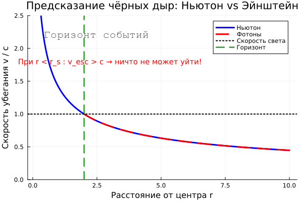
What the graph shows:
- When
r > r_sboth speeds are different, but whenr = r_srelativistic theoryc, and the Newtonian exceedscalready at great distances. - Event horizon
r_smarked with a vertical line. Forr < r_sthe Newtonian curve gives — this is a hint of the impossibility of escape, but only general relativity gives an accurate prediction of a black hole. - Horizontal line
c— the limit of the speed of light.
The following describes the time dilation: — the attitude of one's own time relative to the coordinate time of the falling observer t a remote observer. The redshift formula: — the relative increase in the wavelength of light coming from the vicinity of the black hole.
r_time = range(r_s*1.01, 10, length=300)
time_dilation = @. sqrt(1 - r_s / r_time)           # dτ/dt
redshift = @. 1 / sqrt(1 - r_s / r_time) - 1;       # z = Δλ/λ
p2 = plot(r_time, time_dilation,
     linewidth=3, color=:purple,
     xlabel="Distance r", ylabel="The dt/dt ratio",
     title="Gravitational time dilation",
     legend=:bottomright, grid=true, ylim=(0, 1.1))
hline!(p2, [1.0], ls=:dot, color=:green, label="Away from BH (time is normal)", linewidth=1)
vline!(p2, [r_s], ls=:dash, color=:red, label="Horizon (time stops)", linewidth=2)
annotate!(p2, r_s+0.3, 0.1, text("On the horizon: time stops!", :red, :bold, 9))
annotate!(p2, 5.0, 0.9, text("Away from the Black Hole: time is running normally", :green, 9))
annotate!(p2, 2.0, 0.7, text("At r = 1.5r_s: 1 hour near BH = 1.7 hours on Earth", :purple, 8))
display(p2)
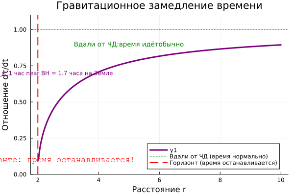
Vertically — (from 0 to 1). Away from the BH, the value tends to 1 (time goes the same way). As you approach the horizon The denominator , therefore — time stops for the falling observer from the point of view of the remote observer. The annotations explain: time "stops" on the horizon, it's normal in the distance, but on the one hour near the Black Hole corresponds to 1.7 hours on Earth. The horizon is marked by a vertical red line, and time stretches indefinitely on it, hence the name event horizon.
p3 = plot(r_time, redshift,
     linewidth=3, color=:orange,
     xlabel="Distance r", ylabel="Redshift z",
     title="Gravitational redshift",
     legend=:topright, grid=true, ylim=(0, 10))
vline!(p3, [r_s], ls=:dash, color=:red, label="Horizon (z → ∞)", linewidth=2)
display(p3)
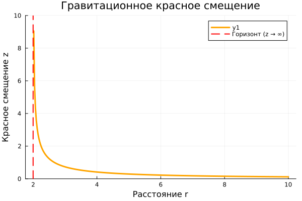
Formula describes how gravity stretches the wavelength of light coming from the vicinity of a black hole. By the denominator tends to zero, so (z\to\infty) — the light turns red infinitely, and the frequency drops to zero. On the chart vertically — z, horizontally is the distance r. The vertical line on r_s shows the horizon where the displacement goes to infinity. Away from the BH (the offset disappears).
Calculations of tidal acceleration are presented below.: , where m is the characteristic size of the object (human height). It shows the difference in the acceleration of free fall between the head and the legs (or between the two ends of the object). The less r, the faster it grows . The conditional destruction threshold is set as (in relative units). From this equation, the radius of the spaghetti is found.: . In the code when the object is being torn apart.
ΔL = 2.0   # human height ~2 m
r_tidal = range(r_s*1.01, 20, length=300)
tidal_accel = @. (2 * G * M / r_tidal^3) * ΔL;
p4 = plot(r_tidal, tidal_accel,
     linewidth=3, color=:darkred,
     xlabel="Distance r", ylabel="Tidal acceleration (relative units)",
     title="Tidal forces — "spaghetti"",
     legend=:topright, grid=true)

r_spaghetti = (2*G*M*ΔL / 100)^(1/3) # Conditional threshold of destruction
vline!(p4, [r_spaghetti], ls=:dot, color=:blue, label="Threshold of destruction")
annotate!(p4, r_spaghetti+0.5, maximum(tidal_accel)*0.8,
          text("For r < $(round(r_spaghetti,digits=2)) the object is being torn apart", :blue, 8))
display(p4)
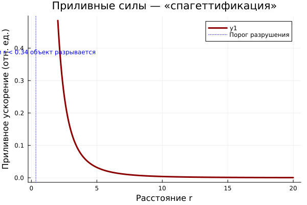
Vertical — tidal acceleration (in relative units), horizontal — distance r from the center of the black hole. The curve increases sharply as it approaches the horizon. The vertical dotted line marks the threshold of destruction. The area to the left of this line is labeled: "the object is being torn apart." The graph clearly demonstrates why spaghetti is most dangerous near small black holes (for supermassive ones, the threshold is inside the horizon, as shown in the table at the end of the example).
The following shows the equation of radial incidence in the Schwarzschild metric for a particle starting from infinity with zero initial velocity ():
where — the proper time of the falling observer. The minus sign indicates movement towards the center.
Function radial_fall_full! calculates this derivative with protection from negative root expression (which may occur when due to numerical errors): if the root expression becomes negative, the derivative is forced to be zero. Integration is performed using the method Tsit5 (adaptive Runge–Kutta of the 5th order) in the proper time interval with an initial condition . The solution is saved in increments saveat=0.05, and the maximum integration step is limited dtmax=0.1.
After obtaining a discrete sequence the coordinate time is calculated from the ratio:
Numerically, this is done using the midpoint rule: for each step, the average radial position is calculated. . Bye , coordinate time increment it is added to the accumulated value. As soon as the particle reaches the event horizon (), accumulation it stops, and then the coordinate time remains constant.
At the end, the values of the proper and coordinate time at the last step of integration are displayed, with a note about the divergence. when approaching the horizon.
function radial_fall_full!(du, u, p, τ)
    r = u[1]
    E = p[1]
    r_s = p[2]
    radicand = E^2 - (1 - r_s/r)
    if radicand < 0
        du[1] = 0.0
    else
        du[1] = -sqrt(radicand)
    end
end
E = 1.0
u0 = [10.0]
τspan = (0.0, 40.0)
prob_rad = ODEProblem(radial_fall_full!, u0, τspan, (E, r_s))
sol_rad = solve(prob_rad, Tsit5(), saveat=0.05, dtmax=0.1)
r_vals = sol_rad[1,:]
τ_vals = sol_rad.t
t_vals = zeros(length(τ_vals))
last_t = 0.0
for i in 2:length(τ_vals)
    r_mid = (r_vals[i-1] + r_vals[i]) / 2
    if r_mid > r_s
        dt_dτ = E / (1 - r_s / r_mid)
        last_t += dt_dτ * (τ_vals[i] - τ_vals[i-1])
        t_vals[i] = last_t
    else
        t_vals[i] = last_t
    end
end
println("The Relativistic fall:")
println("   Proper time to the horizon: $(round(τ_vals[end], digits=2))")
println("   Coordinate time to the horizon: $(round(t_vals[end], digits=2)) (diverges)")
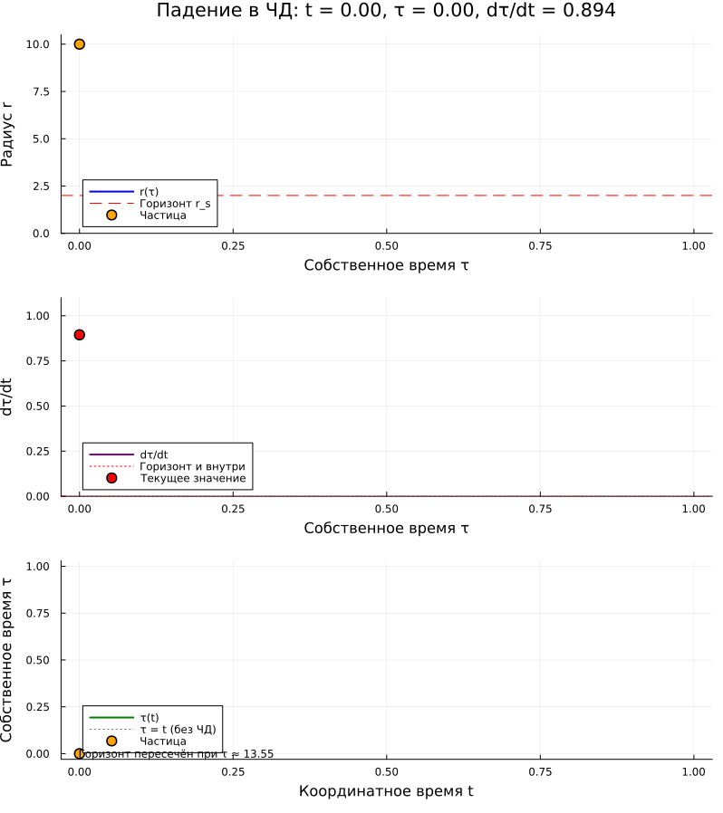
The following is an interactive visualization of the body's approach to the black hole.
The first graph (Radial incidence) shows how the distance from the falling object to the center of the black hole decreases with the passage of its own time (time according to the falling object's clock). The horizontal red dotted line is the event horizon. It can be seen that the object crosses the horizon in a finite proper time and continues to fall towards the center.
The second graph (Time Dilation) shows the ratio of the rate of the falling clock to the rate of the clock of the remote observer. The closer to the horizon, the more time slows down for the falling person from the point of view of an external observer. At the horizon itself and inside it, this ratio drops to zero – for a remote observer, time stops.
The third graph (Time Relation) compares the coordinate time (according to the clock of the remote observer) and the falling person's own time. The dotted gray line shows how they would match up in the absence of a black hole. The real green curve shows that as we approach the horizon, our own time lags further and further behind. After crossing the horizon, the coordinate time practically stops growing (tends to a finite limit), while the proper time continues to increase. The annotation in the lower left corner indicates that the horizon intersects at its own time of approximately 13.55.
dilation_vals = [r > r_s ? sqrt(1 - r_s/r) : 0.0 for r in r_vals]

anim = @animate for i in 1:5:length(τ_vals)
    r_cur = r_vals[i]
    τ_cur = τ_vals[i]
    t_cur = t_vals[i]
    dil_cur = dilation_vals[i]
    title_str = @sprintf "Drop in BH: t = %.2f, τ = %.2f, dtt/dt = %.3f" t_cur τ_cur dil_cur

    p1 = plot(τ_vals[1:i], r_vals[1:i],
              color=:blue, linewidth=2,
              label="r(τ)",
              xlabel="Proper time of τ",
              ylabel="Radius r",
              legend=:bottomleft,
              title=title_str,
              ylim=(0, maximum(r_vals)+0.5))
    hline!(p1, [r_s], ls=:dash, color=:red, label="Horizon r_s")
    scatter!(p1, [τ_cur], [r_cur], color=:orange, ms=6, label="Particle")

    p2 = plot(τ_vals[1:i], dilation_vals[1:i],
              color=:purple, linewidth=2,
              label="dτ/dt",
              xlabel="Proper time of τ",
              ylabel="dτ/dt",
              legend=:bottomleft,
              ylim=(0, 1.1))
    hline!(p2, [0], ls=:dot, color=:red, label="The horizon and inside")
    scatter!(p2, [τ_cur], [dil_cur], color=:red, ms=6, label="Current value")

    p3 = plot(t_vals[1:i], τ_vals[1:i],
              color=:green, linewidth=2,
              label="τ(t)",
              xlabel="Coordinate time t",
              ylabel="Proper time of τ",
              legend=:bottomleft)
    plot!(p3, t_vals[1:i], t_vals[1:i], ls=:dot, color=:gray, label="τ = t (without BH)")
    scatter!(p3, [t_cur], [τ_cur], color=:orange, ms=6, label="Particle")
    x_min = minimum(t_vals[1:i])
    y_min = minimum(τ_vals[1:i])
    annotate!(p3, x_min + 0.05*(maximum(t_vals[1:i])-x_min),
                   y_min + 0.05*(maximum(τ_vals[1:i])-y_min),
              text("The horizon is crossed at τ ≈ 13.55", :black, :left, 8))

    plot(p1, p2, p3, layout=(3,1), size=(800, 900))
end

gif(anim, "relativistic_fall_full.gif", fps=20)
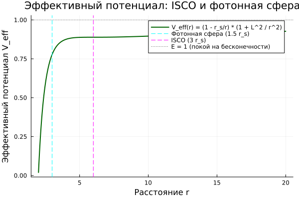
Below is a graph of the effective potential. It shows how the "energy barrier" depends on the distance to the black hole for a particle moving in orbit. Vertically is the effective potential energy, horizontally is the distance. The minima on the curve correspond to stable circular orbits, while the maxima correspond to unstable ones.
- Photon sphere (blue vertical line) — the distance at which light can travel in a circular orbit around a black hole. This orbit is unstable: the slightest disturbance and the photon will either fall into the hole or fly away.
- ISCO (the last stable circular orbit) (pink vertical line) is the innermost radius at which stable circular motion of a massive particle is possible. Closer to the hole, any circular orbit becomes unstable, and the particle quickly falls inside. ISCO plays a key role in astrophysics: it is at this radius that the accretion disk ends, and matter begins to fall irrevocably into the black hole, releasing enormous energy.
- The horizontal gray line is the energy level of a particle at rest at infinity. Where this line intersects with the potential curve, there are possible turning points of movement.
r_photon = 1.5 * r_s
r_ISCO = 3.0 * r_s

println("Additional orbits:")
println("   Photonic sphere: r = $r_photon")
println("   Last Stable Orbit (ISCO): r = $r_ISCO")
L_isco = 2.0 * sqrt(3) * M
r_pot = range(r_s+0.01, 20, length=500)
V_eff = @. (1 - r_s/r_pot) * (1 + L_isco^2 / r_pot^2)

p5 = plot(r_pot, V_eff,
     label="V_eff(r) = (1 - r_s/r) * (1 + L^2 / r^2)",
     linewidth=2, color=:darkgreen,
     xlabel="Distance r", ylabel="Effective potential of V_eff",
     title="Effective potential: ISCO and the photonic sphere",
     legend=:topright, grid=true)
vline!(p5, [r_photon], ls=:dash, color=:cyan, label="Photonic sphere (1.5 r_s)")
vline!(p5, [r_ISCO], ls=:dash, color=:magenta, label="ISCO (3 r_s)")
hline!(p5, [1.0], ls=:dot, color=:gray, label="E = 1 (rest at infinity)")
display(p5)
savefig("effective_potential.png")
println(" Graph 5 saved and displayed: efficie_potential.png")
Below is a table of real objects, which we referred to above, the table shows four types of black holes of different masses: stellar mass (10 solar masses), Sagittarius A* (a supermassive hole in the center of our Galaxy, 4.3 million solar masses), M87* (6.5 billion solar masses) and TON 618 (one of the most massive known holes is 66 billion solar masses).
Calculated for each object:
- The Schwarzschild radius
r_s(event horizon) in kilometers. - Tidal radius — the distance at which tidal forces tear apart an object measuring 2 meters (human height) with an acceleration equal to that of the earth .
- Minimum safe distance — the maximum of the tidal radius and (in order not to go over the horizon).
- The time dilation at this minimum distance is how many times 1 hour near the hole is longer for a remote observer.
G_si = 6.67430e-11
c_si = 299792458
M_sun = 1.989e30
ΔL = 2.0          # human height, m
g_earth = 9.8     # m/s2

r_s_km(mass_solar) = 2 * G_si * (mass_solar * M_sun) / c_si^2 / 1000 # Schwarzschild radius in km
function r_tidal_km(mass_solar)
    M_kg = mass_solar * M_sun
    r_m = (2 * G_si * M_kg * ΔL / g_earth)^(1/3)
    return r_m / 1000
end
function dilation_factor(r_km, r_s_km)
    if r_km <= r_s_km
        return Inf
    else
        return 1 / sqrt(1 - r_s_km / r_km)
    end
end

objects = [
    ("BH of stellar mass", 10),
    ("Sagittarius A*", 4.3e6),
    ("M87*", 6.5e9),
    ("TON 618", 6.6e10)
]

rows = []
for (name, mass) in objects
    rs = r_s_km(mass)
    r_tidal = r_tidal_km(mass)
    r_min = max(r_tidal, rs * 1.0001)
    dilation = dilation_factor(r_min, rs)
    push!(rows, (name, mass, rs, r_tidal, r_min, dilation))
end

df = DataFrame(
    Symbol("An object") => [row[1] for row in rows],
    Symbol("M (M☉)") => [row[2] for row in rows],
    Symbol("r_s (km)") => [round(row[3], sigdigits=4) for row in rows],
    Symbol("r_tidal (km)") => [round(row[4], sigdigits=4) for row in rows],
    Symbol("r_min (km)") => [round(row[5], sigdigits=4) for row in rows],
    Symbol("Deceleration (1 hour → hours)") => [row[6] for row in rows]
)

println("Table: for each object, the minimum distance is indicated at which it is possible to be without being torn apart by tidal forces (but no closer than 1.0001 r_s), and the corresponding time dilation.")
println(df)
Key findings of the table:
- For a stellar-mass black hole, the tidal radius (about 8,150 km) is significantly larger than the horizon (about 30 km). Therefore, the astronaut will be torn apart by tidal forces long before reaching the horizon. The time dilation at a safe minimum is small (only 1,002 times).
- For supermassive holes (Sagittarius A*, M87*, TON 618), the picture is reversed: the tidal radius lies deep inside the horizon. This means that the horizon can be crossed without feeling the spaghetti — the tidal forces at the edge of the black hole are very weak. However, the time dilation at the minimum distance (which in this case is limited by the horizon itself) is enormous: 1 hour near the horizon stretches to 100 hours for an external observer (coefficient 100). This follows from the fact that the minimum distance is almost equal to
r_s, and the denominator it becomes very small.
Conclusion
This article is a practical introduction to modeling black holes in the framework of general relativity. It illustrates that the Newtonian theory of gravity uses the escape velocity formula. , predicts: if an object is massive and compact enough, then when the escape velocity exceeds the speed of light, and light cannot leave such a "dark star" (Michell's idea, 1783). However, this is only one side of the issue, since in Newtonian physics light has no mass and should not obey gravity in the same sense. Einstein's general theory of relativity (1915) gives a strict description: gravity is a curvature of space-time, and the Schwarzschild metric (1916) predicts the event horizon. beyond which nothing, not even light, can come out. In addition, general relativity predicts qualitatively new effects: gravitational time dilation (time on the horizon stops), redshift, tidal forces ("spaghetti"), as well as the existence of a photonic sphere and the last stable orbit of ISCO. In the code, we visually compare Newtonian and relativistic escape velocities, demonstrating that only general relativity gives the correct value of the horizon radius and explains the observed phenomena.