Credit Calculator

This article discusses the software implementation of a universal credit calculator. The main focus is on the internal structure of the module, key algorithms, data structures, and approaches that ensure accuracy, flexibility, and ease of integration with the interface of code cell masks.

1. General architecture

The module is built around a central function CreditCalculator, which acts as a facade for two independent calculation algorithms: annuity and differential. All auxiliary functions are encapsulated, and the returned data is standardized in the form of named tuples (NamedTuple) and tables DataFrame from the package DataFrames.jl.

Main components:

• CreditCalculator is a dispatcher that validates input parameters and selects a method.
• calculate_annuity / calculate_differentiated – pure functions that implement financial formulas.
• compare_payment_types is a service function for comparing two schemes.
• print_payment_schedule is an output function (side‑effect) for formatted display.

This design provides a separation of responsibilities: calculations are separated from input/output, and the returned structures can be used for subsequent analysis or visualization.

2. Input parameters and validation

Function CreditCalculator uses named arguments with typing, which increases the readability of the code and allows you to set values in any order.:

function CreditCalculator(; amount::Float64, rate::Float64, term::Int, 
                          payment_type::String="annuity", 
                          start_date::Date=today(), 
                          loan_type::String="consumer")

Validation is performed at the entrance:

• Verification that the amount, bid and term are positive.
• Checking that payment_type belongs to the set {"annuity", "differentiated"}.

This prevents incorrect calculations at an early stage and provides clear error messages.

3. Calculation algorithms

3.1. Annuity payments

The annuity ratio is calculated using the classical formula:

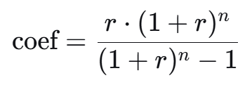
where r = the rate / (100 * n) is the monthly interest rate, and n is the term in months.

Implementation features:

• The monthly payment is calculated as amount * coef.
• For each month, the interest on the balance and the repayment amount of the principal debt are calculated.
• Correction of the last payment: due to rounding, an error may accumulate, therefore, at the last step, the amount of the principal debt is forcibly set equal to the balance, and the payment is recalculated. This ensures that the final balance will be zero.
• All amounts are rounded to two decimal places using round(..., digits=2).
• Data is accumulated in DataFrame by making consecutive calls push!.

3.2. Differentiated payments

Here, the monthly portion of the principal debt is fixed:

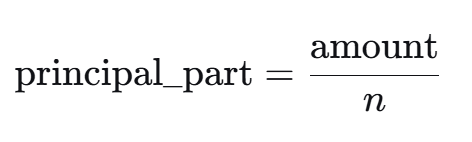
The monthly interest is calculated from the current balance. The payment decreases linearly.

Features:

• Unlike an annuity, no adjustment of the last payment is required, since the balance is reset exactly after the last payment (provided that the amount is accurately divided by an integer number of months).
• For the convenience of comparison, the first and last payments are saved.
• When building the table principal_part It is rounded only during output, but full precision is used in calculations to avoid accumulation of errors.

4. Structures of the returned data

Both options return NamedTuple with the same fields, which allows you to write generalized code.:

(loan_type = ..., payment_type = ..., amount = ..., rate = ..., term = ...,
 total_payment = ..., total_interest = ..., overpayment_percent = ...,
 payments_table = DataFrame(...))

There is an additional field for an annuity monthly_payment, for the differentiated – first_payment and last_payment. This structure is convenient for subsequent processing.

Payment table payments_table contains columns:

• month – month number (Int)
• date – date of payment (Date)
• payment – payment amount (Float64)
• principal – the part going to the main debt (Float64)
• interest – the percentage portion (Float64)
• remaining_debt – debt balance after payment (Float64)

Using DataFrame allows you to apply all the features of the package to the results. DataFrames.jl (filtering, aggregation, merging) without additional transformations.

5. Processing boundary conditions

The following edge cases are provided in the code:

• Zero or negative parameters – an error is thrown.
• Incorrect payment type is an error with a clear message.
• For an annuity at term = 1 The annuity ratio formula is still working, and the correction of the last payment guarantees accuracy.
• With a differentiated calculation principal_part It is not rounded to avoid accumulating errors over long periods of time.

6. Testing and usage examples

The four examples presented in the sketch serve not only as demonstrations, but also as implicit tests. Let's look at what aspects they check.

Example 1. Annuity loan

• Checks the correctness of the calculation of the annuity coefficient.
• Makes sure that the last payment is adjusted and the balance is reset to zero.
• Demonstrates rounding to pennies.

Example 2. Mortgage (differentiated payments)

• Checks the work with dates (transfer start_date and calculating dates via Dates.Month).
• Outputs the full graph via print_payment_schedule, confirming that the formatting is correct.
• Compares the first and last payments to ensure a linear decrease.

print_payment_schedule - payment schedule output. Function print_payment_schedule accepts the result as input CreditCalculator and outputs a formatted report. Its implementation uses string manipulation (rpad, Dates.format) and iterate through the lines DataFrame. This approach separates the representation from the calculation logic. If necessary, it is easy to replace the output with another one (for example, in a file or HTML).

Example 3. Comparison of payment types

• Checks that the function compare_payment_types returns a structure with three fields.
• Compares the numerical values of overpayments, confirming that the annuity provides a slightly higher overpayment with the same parameters.

compare_payment_types - the comparison function, it calls twice CreditCalculator with different payment_type and generates the final table. The table is created as DataFrame with three columns: indicator, values for annuity and for differentiated. This demonstrates how the results of a single module can be used to build more complex reports.

Example 4. Analysis of payment table data

• Shows how to extract the first five lines (first).
• Calculates the maximum, minimum, and amount of interest – thereby verifying that the columns payment and interest they contain correct numeric data.
• Demonstrates that the returned DataFrame It is fully functional and can be used for statistical analysis.

Conclusion

The developed module demonstrates the effective use of Julia's features: multiple dispatching through named arguments, type safety, and convenient data structures (NamedTuple, DataFrame) and a functional composition. This approach makes it easy to maintain the code, add new types of calculations (for example, taking into account early repayment) and integrate the calculator into larger financial applications. The test cases simultaneously serve as documentation and confirmation of the correctness of the algorithms.