Modeling of gas systems
Intended application areas
The Gas library contains basic elements such as cameras, sensors, and sources [1], as well as holes and pneumomechanical transducers [2]. Use these blocks to model gas systems in applications such as:
-
Pneumatic control of mechanical systems;
-
Transportation of natural gas through pipeline networks;
-
Gas turbines for energy production;
-
Air cooling of thermal components.
The properties of the gas are set in the connected circuit using the block Gas Properties (G). This block allows you to select one of three gas models: ideal gas, semi-ideal gas, or real gas (see Gas models).
Unless explicitly stated otherwise, all pressures and temperatures used in the modeling of gas systems are static pressure and static temperature.
Network variables
The potential variables (Across variables) are pressure and temperature, and the flow variables (Through variables) are mass flow and energy flow. Note that this choice corresponds to a pseudo-connected graph, since the product of pressure and mass flow is not a power.
Gas models
Library Gas Supports ideal gas, semi-ideal gas, and real gas within the same gas domain, allowing a wide range of modeling requirements to be met. The three gas models provide a compromise between speed and simulation accuracy. They also allow for step-by-step model development: start with a simple model that requires minimal information about the working gas, and then develop it as more detailed data on the properties of the gas becomes available.
The gas model is selected using the block Gas Properties (G), which sets the properties of the gas in the connected circuit.
The following table shows the different assumptions for each gas model.
-
The equation of state for thermal properties describes the dependence of density on temperature and pressure.
-
The equation of state for caloric properties describes the dependence of the specific heat capacity on temperature and pressure.
-
Transport properties describe the dependence of dynamic viscosity and thermal conductivity on temperature and pressure.
| The gas model | The thermal equation of state | The caloric equation of state | Transport properties |
|---|---|---|---|
The ideal gas |
The Ideal Gas Law |
The constant |
The constant |
Semi-ideal gas |
The Ideal Gas Law |
One-dimensional temperature interpolation table |
One-dimensional temperature interpolation table |
Real gas |
Two-dimensional interpolation table of temperature and pressure |
Two-dimensional interpolation table of temperature and pressure |
Two-dimensional interpolation table of temperature and pressure |
The ideal gas law is implemented in the fundamental library Gas as follows:
where
-
— pressure;
-
— the coefficient of compressibility;
-
— density;
-
— specific gas constant;
-
— temperature.
Compressibility factor It is usually a function of pressure and temperature. It takes into account the deviation from the behavior of an ideal gas. Gas is ideal when . In models of ideal and semi-ideal gases It must be constant, but not necessarily equal. 1. For example, if you are modeling an imperfect gas ( ), but the temperature and pressure of the system change slightly, you can use the ideal gas model and set the appropriate value. . The following table shows the values of the compressibility factor for various gases at temperature 293.15 K and pressure 0.101325 MPa:
| Gas | Compressibility factor |
|---|---|
Dry air |
|
Carbon dioxide |
|
Oxygen |
|
Hydrogen |
|
Helium |
|
Methane |
|
Natural gas |
|
Ammonia |
|
R-134a |
|
Using an ideal gas model with a constant value adjusted depending on the type of gas and operating conditions, it avoids the additional complexity and computational costs associated with the transition to a semi-ideal or real gas model.
The ideal gas model is a good initial choice when modeling a gas network because it is simple, computationally efficient, and requires a limited amount of information about the working gas. It is correct for monatomic gases and, as a rule, is quite accurate for gases such as dry air, carbon dioxide, oxygen, hydrogen, helium, methane, natural gas, etc., under standard conditions.
When the gas network operates near the boundary of the saturation region or in a very wide temperature range, the working gas may exhibit moderate imperfect behavior. In this case, after successful modeling of the gas network using the ideal gas model, it is necessary to switch to the semi-ideal gas model.
Finally, we should switch to the real gas model if it is expected that the working gas will exhibit highly imperfect behavior, for example, heavy gases with large molecules. This model is the most computationally expensive and requires detailed information about the working gas, since it uses two-dimensional interpolation for all properties.
Gas volume units
The components in the gas domain are modeled using control volumes. The reference volume covers the gas inside the component and separates it from the environment and other components. Gas flows and heat flows through the control surface are represented by ports. The volume of gas inside the component is represented by an internal node that sets the pressure and temperature of the gas inside the component.
The following blocks are in the library Gas they belong to the described group. In the case of blocks Controlled Reservoir (G) and Reservoir (G) it is assumed that the volume is infinitely large.
| Block | Gas volume |
|---|---|
Finite |
|
Finite |
|
Finite |
|
Finite |
|
Infinite |
|
Infinite |
Other components have a relatively small volume of gas, so the residence time of the gas inside the component is negligible. Such components are considered quasi-stationary and do not have an internal node.
The reference node and the rules for building the network
Unlike mechanical and electrical domains, where each topologically isolated circuit within the domain must contain at least one support unit, gas networks have different network construction rules.
The gas volume units contain an internal unit that provides the pressure and temperature of the gas inside the component and, therefore, serves as a reference unit for the gas network. Each connected gas network must have at least one reference node. This means that each connected gas network must have at least one of the blocks listed in the Gas volume units section. In other words, a gas network that does not contain a volume of gas is an incorrectly constructed gas network.
The Fundamental Library Gas contains a block Absolute Reference (G) but, unlike other domains, it is not used to build a network of gas chains. Block assignment Absolute Reference (G) it consists in providing a reference value for the block Absolute Pressure & Temperature Sensor (G). However, this block contains an implicit reference node, which makes the use of the block Absolute Reference (G) with a block Absolute Pressure & Temperature Sensor (G) unnecessary. If you use the block Absolute Reference (G) in another place of the gas network, this will cause a modeling error, since the pressure and temperature of the gas cannot be equal to absolute zero.
Initial conditions for blocks with a finite volume of gas
This section discusses the specific initialization requirements for blocks modeled with a finite volume of gas. These blocks are listed in the Gas volume units section.
The state of the gas volume changes dynamically through the flows of mass and energy through the compounds. The time constants depend on the compressibility and heat capacity of the gas volume.
The state of the gas volume is represented by differential variables in the internal node of the block. As differential variables, they require setting initial conditions before starting the simulation. The settings window for each block modeled with a finite volume of gas contains a group of parameters Initial Targets, which lists three variables:
-
Pressure of gas volume;
-
Temperature of gas volume;
-
Density of gas volume.
By default Pressure of gas volume and Temperature of gas volume they have a high priority, and their target values are equal to the standard values (0.101325 MPa and 293.15 K). You can adjust the target values so that they correspond to the initial state of the gas volume for the unit. Parameter Density of gas volume has a default priority None since only the initial conditions of two of the three variables are needed to fully determine the initial state of the gas volume. An alternative way to set the initial conditions is to change the priority of the parameter. Density of gas volume set to high with the appropriate target value, and then change the priority of the parameter Pressure of gas volume or Temperature of gas volume on the value None.
It is important that only two of the three variables have priority. High for each unit with a finite volume of gas. Imposing high-priority constraints on all three variables redefines the system, as a result of which the solver cannot find an initial solution that satisfies the desired initial values. Conversely, imposing a high priority constraint on only one variable makes the system undefined, and the solver can define variables with arbitrary and unintended initial values.
In blocks modeled with an infinitely large volume of gas, the state of the gas volume is considered quasi-stationary, and there is no need for initial conditions.
Critical flow mode
Gas flow through the blocks Local Restriction (G) or Pipe (G) It may enter critical mode. This mode occurs when the flow velocity reaches the local speed of sound. After reaching the critical mode, the flow velocity in the critical section can no longer increase. However, the mass flow rate may continue to increase if the gas density increases. This can be achieved, for example, by increasing the pressure before the critical section. The peculiarity of the critical mode in the gas network is that the mass flow through the branch containing the critical flow unit is completely determined by the inlet pressure and temperature. As long as the critical mode is maintained, this critical mass flow rate is independent of any pressure changes at the flow outlet.
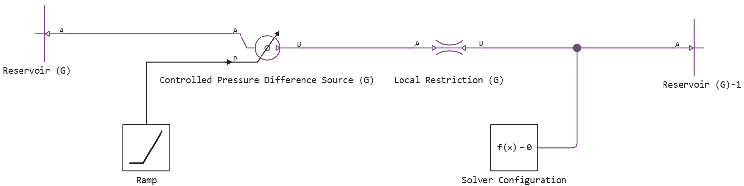
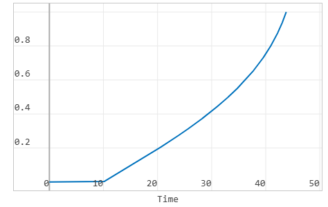
The following model illustrates the occurrence of a critical flow regime (throttled flow). In this model, the block Ramp it has a slope 0.005 and the start time 10. All other blocks have default parameter values. The simulation time is 50 c. When simulating the pressure in the port A of the block Local Restriction (G) increases linearly from atmospheric pressure, starting from 10 c. The pressure in port B is fixed at atmospheric pressure.
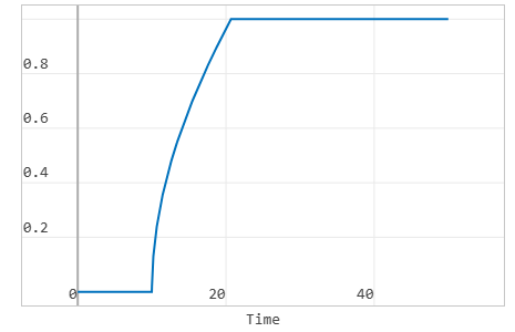
The following figures show the simulation data recorded for the block Local Restriction (G). The Mach number at the restriction point reaches 1 In about a month 20 c, which indicates throttling of the flow.
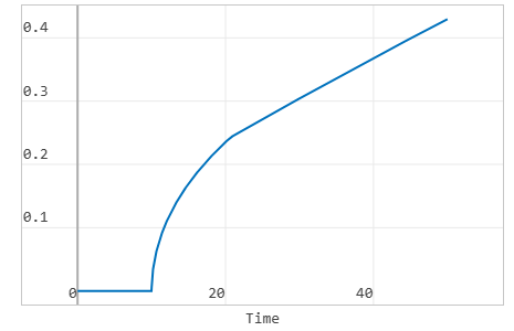
The mass flow rate before flow throttling exhibits typical quadratic behavior with respect to an increasing pressure difference. However, the mass flow after throttling becomes linear, since the throttled mass flow depends only on the inlet pressure and temperature, and the inlet pressure increases linearly.
The fact that the mass flow rate with throttling depends only on the inlet conditions may lead to incompatibility with the unit. Controlled Mass Flow Rate Source (G), connected after the block with throttling. Consider the model shown in the following figure, which contains a block Controlled Mass Flow Rate Source (G) instead of a block Controlled Pressure Difference Source (G).
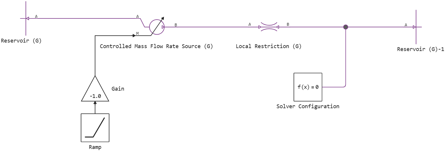
If the source specifies an increasing mass flow rate from left to right through the block Local Restriction (G) the simulation will be successful even if the flow becomes critical because the block Controlled Mass Flow Rate Source (G) it will be located in front of the block with throttling. However, in this model, the block Gain reverses the flow direction so that the block Controlled Mass Flow Rate Source (G) it is located at the outlet of the flow from the block with throttling. Pressure in front of the unit Local Restriction (G) it is fixed at the atmospheric pressure level. Therefore, in this situation, the mass flow rate with throttling is constant. As the set mass flow rate increases, it will eventually become greater than this constant throttled flow rate. At this point, the set and throttled mass costs cannot be matched, and the simulation will fail. Viewing the recorded simulation data in Engee shows that the simulation completes with an error exactly at the moment when the Mach number reaches 1 and the flow becomes throttled.
In general, if there is a possibility of a critical mode in the model, use pressure sources rather than mass flow sources. If the model contains blocks of mass flow sources and the simulation fails, use signal visualization to study the Mach number graph and check its variables in all blocks Local Restriction (G) and Pipe (G) connected along the same branch as the mass flow source. If a simulation failure occurs when the Mach number reaches 1 It is likely that the source of the mass flow at the outlet is trying to set a mass flow that exceeds the possible critical mass flow.
The Mach number variable for the restriction blocks is called Mach. Block Pipe (G) It has two variable Mach numbers: Mach_a and Mach_b representing the Mach number at port A and port B, respectively.
The occurrence of backflow
The gas flow through the circuit transfers energy from one volume of gas to another volume of gas. Therefore, the energy flow between two connected units depends on the flow direction. If gas flows from block A to block B, then the energy flow between the two blocks is determined by the specific total enthalpy of block A. Conversely, if gas flows from block B to block A, then the energy flow between the two blocks is determined by the specific total enthalpy of block B. To smooth out the transition and increase the stability of the simulation, the energy flow also includes a contribution based on the difference in the specific total enthalpies of the two blocks at low mass flow rates. The smoothing area is controlled by the parameter Mach number threshold for flow reversal the block Gas Properties (G).
The consequence of this approach is that the temperature of the node between the two connected blocks is the temperature of the volume of gas located upstream from this node. If two or more streams converge at a node, then the temperature at the node is a weighted average temperature based on the ideal mixing of the merging gas streams.
Modeling stability can be difficult for models that experience rapid changes in flow direction and large temperature differences between blocks. Rapid changes in flow direction may result from low flow resistance (e.g., short pipes) between large volumes of gas. Large temperature differences may be the result of energy added by sources to maintain large pressure differences in a low-heat model. In such models, it may be necessary to increase the parameter value. Mach number threshold for flow reversal to avoid simulation failure.
The cross-sectional area of the block ports
Many blocks in the gas domain allow you to set the cross-sectional area at the input and output ports as a block parameter. It is recommended to specify the same cross-sectional area for interconnected ports. For example, if the port A of the block is Constant Volume Chamber (G) connected to the unit Pipe (G), set for the parameter Cross-sectional area at port A the block Constant Volume Chamber (G) the same value as for the parameter Cross-sectional area the block Pipe (G).
Differences in the areas of the connected ports can lead to unexpected temperature fluctuations, especially for high-speed streams where the Mach number is close to 1.