OFDM Oversampled Signal Model
In this example, we will consider the OFDM oversampled signal model (Orthogonal frequency-division multiplexing, a digital modulation technology using a large number of closely spaced orthogonal subcarriers, or multiplexing). The model allows you to see a combination of several modulations. This example also uses an RMS unit that measures an OFDM-modulated signal with noise superimposed on it, scaled by a value proportional to the number of active subcarriers relative to the size of the FFT (Fast Fourier transform) to confirm that the signal power is approximately one.
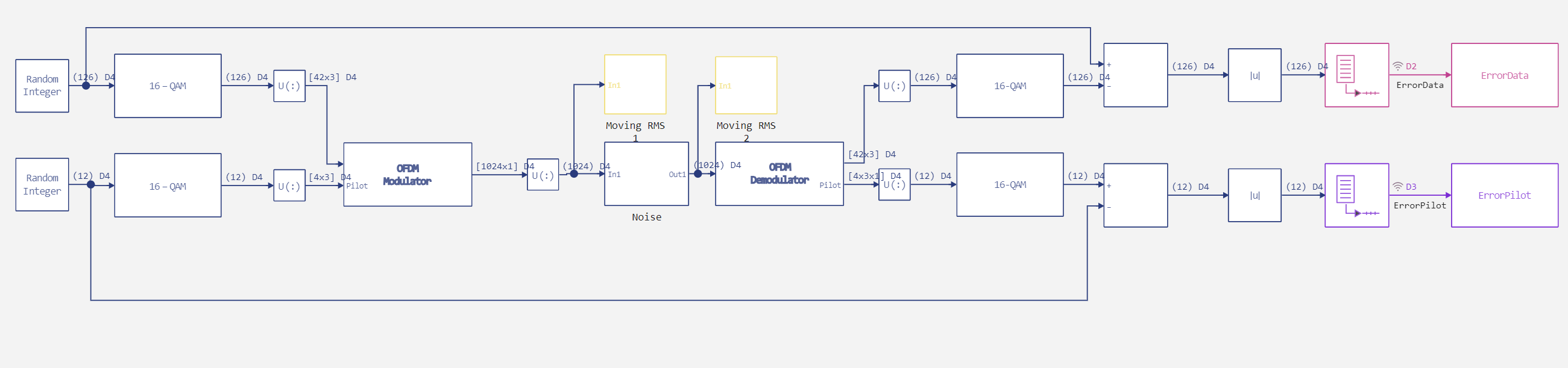
The model is based on the following principle.
- A random integer data set and pilot input characters are generated.
- 16-QAM modulates data and pilot symbols.
- OFDM modulates the QAM-modulated signal. A pair of OFDM modulators and demodulators processes three symbols with different subcarrier indexes of the pilot signal and cyclic prefix lengths for each symbol. The OFDM signal contains data and pilots that the model generates at a frequency four times the sampling rate.
- Next, we apply amplitude distortion to each frame, which significantly changes the signal strength.
- After that, OFDM demodulates and outputs the data and pilots separately.
- 16-QAM demodulates data and pilot symbols.
- After that, we find the difference between the input and output.
The figure below shows the implemented model.
Next, initialize the model parameters.
M = 16;              # The order of modulation
nfft = 64;           # FFT Length
NumSymbols=3;        # Number of characters OFDM
osf=4;               # The oversampling factor
ngbc = [9;8];        # Number of protective range carriers
insertdcnull = true;  # The presence of a DC-zero subcarrier
addpilotport = true;  # Pilot's presence
Noise_power = 10; # Noise power
# Indexes of pilot subcarriers
pscindx = [[12;26;40;54] [14;28;38;52] [12;26;40;54]];
cplen = [16; 32; 16];  # CyclicPrefixLength
# Samples per frame for data
spf_data = NumSymbols * (nfft-sum(ngbc)-size(pscindx,1)-insertdcnull)
# Selections per frame for the pilot
spf_pilot = NumSymbols * size(pscindx,1)
# Number of active subcarriers
nasc = nfft-sum(ngbc)+insertdcnull;
After declaring the model parameters, initialize the model startup function and run the model itself.
# Enabling the auxiliary model launch function.
function run_model( name_model)

    Path = (@__DIR__) * "/" * name_model * ".engee"

    if name_model in [m.name for m in engee.get_all_models()] # Checking the condition for loading a model into the kernel
        model = engee.open( name_model ) # Open the model
        model_output = engee.run( model, verbose=true ); # Launch the model
    else
        model = engee.load( Path, force=true ) # Upload a model
        model_output = engee.run( model, verbose=true ); # Launch the model
        engee.close( name_model, force=true ); # Close the model
    end
    sleep(5)
    return model_output
end

run_model("OFDM_Signal_and_QAM") # Launching the model.
Now let's analyze the recorded dates.
ErrorData = collect(ErrorData);
ErrorPilot = collect(ErrorPilot);
RMSinp = collect(RMSinp);
RMSout = collect(RMSout);

ErrorData = ErrorData.value;
ErrorPilot = ErrorPilot.value;
RMSinp = RMSinp.value;
RMSout = RMSout.value;
plot([real(RMSinp),real(RMSout)], title="RMS", label=["Before the noise was applied" "After applying noise"])
As we can see, the signal strength varies from frame to frame. Now let's look at the difference between the input and output data.
plot([ErrorData,ErrorPilot], title="The difference between inputs and outputs", label=["Data" "Pilots"])
According to the graph, the error is zero, but to make sure of this, we will find the total error.
println("Total difference between input and output data: " * string(sum(ErrorData)))
println("Total difference between entry and exit pilots: " * string(sum(ErrorPilot)))
Conclusion
In this example, we have analyzed and demonstrated the possibilities of using several types of modulations in communication systems. This approach is very much in demand in this field of activity.