Slow-scan television
In this example, we will consider the image transmission protocol based on Slow Scan Television (SSTV), which is slow—scan television or low-frame television. It is a unique and flexible image transmission protocol that is ideally suited for narrow-band communication channels. The variability of SSTV allows you to adapt the transmission to specific conditions, and the simplicity of its implementation makes it popular among radio amateurs. However, due to the low transfer rate, SSTV is not suitable for tasks requiring high speed or high image quality.
This model is not tied to any communication standard implemented in practice, and primarily describes the technologies and methods that we can apply in Engee for such systems.
The general principle of SSTV is to transmit static images over narrow-band communication channels such as radio channels. The process can be divided into several stages: image encoding, modulation, transmission, reception, demodulation and decoding.
Next, let's move on to the implemented model.
Model analysis
The following logic is implemented at the input of the model: we read the image into the model using the Images library and normalize the image.
.png)
using Images

path_img = "$(@__DIR__)/img.jpg"
inp_img = imrotate(Gray.(load(path_img)), deg2rad(-90))

S = size(inp_img)
println("Input image size: $(S))")
In this example, all work with the image will be carried out in the format of gray shadows of the representation. If we consider Julia representations, this means that pixels are encoded in the range from 0 to 1, where 0 is black and 1 is white.
Gray.([1,0])

Now let's move on to the next block, the interleaving block. Interleaving is a technique used in data transmission systems to increase error tolerance. The basic idea is to change the order of the data before transmission, and then neighboring bits or characters will be separated in the stream.
.png)
This block is implemented using the Engee Function. At the input, it has the number of interleaving groups and the input signal itself.
The interleaving formula:
index = mod((i - 1) * n, N) + div(i - 1, div(N, n)) + 1
The depersonalization formula:
index = mod((i - 1), n) * div(N, n) + div(i - 1, n) + 1
These formulas ensure that the index does not exceed the limits of the array, since the mod operation is used to limit the index within N.
Let's compare the formulas themselves.
-
There is a difference in calculating the position within the group.
In the first formula, the position within the group is calculated as follows: mod((i−1),n).
In the second formula, the position within the group is calculated as follows: mod((i−1)×n,N). -
There are also differences in the calculation of the group number.
In the first formula, the group number is calculated as follows: div(i−1,n).
In the second formula, the group number is calculated in this way: div(i−1,div(N,n)).
That is, as we can see, they are mutually reversible. Next, let's look at a simple example of the interleaving we implemented.
L = 4
data_in = collect(1:L)
n = 2 # parts of the array
println("Initial data: ", data_in)

# The interleaving function
N = length(data_in)
interleaved_data = similar(data_in)

for i in 1:N
    index = mod((i - 1) * n, N) + div(i - 1, div(N, n)) + 1
    interleaved_data[i] = data_in[index]
end

println("Interleaved data: ", interleaved_data)

# The interleaving function
N = length(interleaved_data)
deinterleaved_data = similar(interleaved_data)

for i in 1:N
    index = mod((i - 1), n) * div(N, n) + div(i - 1, n) + 1
    deinterleaved_data[i] = interleaved_data[index]
end

println("Deperjected data: ", deinterleaved_data)
As we can see, the algorithm is working correctly. Now let's set the number of groups for our model.
num = 400 # Number of groups
println("Number of values in the group: $((S[1]*S[2])/num)")
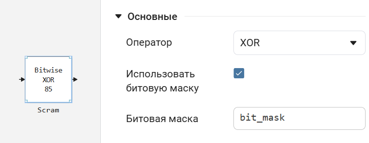
The next block we use is XOR. This operation is reversible and allows you to implement a simple version of the scrambler.
.png)
A scrambler (from the English scramble — to encrypt, to mix) is a software or hardware device that performs scrambling, that is, the reversible transformation of a digital stream without changing the transmission rate in order to obtain the properties of a random sequence. After scrambling, the occurrence of "1" and "0" in the output sequence is equally likely.
Next, we will set the bitmask for our scrambler.
bit_mask = 0b01010101 # max 8 bit
println("bit_mask: $bit_mask")
The next blocks that we will consider are a bundle of 16—FSK modulation and automatic gain control (AGC).
FSK is a modulation method in which digital data (bits) are transmitted by changing the frequency of the carrier signal. Each bit value (0 or 1) or group of bits corresponds to a certain frequency. 16-FSK is an extension of FSK, which uses 16 different frequencies to transmit 4 bits of data simultaneously.
Bit and number matching table for 16-FSK:
| A combination of bits | Number |
|---|---|
[0, 0, 0, 0] |
1 |
[0, 0, 0, 1] |
3 |
[0, 0, 1, 0] |
5 |
[0, 0, 1, 1] |
7 |
[0, 1, 0, 0] |
9 |
[0, 1, 0, 1] |
11 |
[0, 1, 1, 0] |
13 |
[0, 1, 1, 1] |
15 |
[1, 0, 0, 0] |
-1 |
[1, 0, 0, 1] |
-3 |
[1, 0, 1, 0] |
-5 |
[1, 0, 1, 1] |
-7 |
[1, 1, 0, 0] |
-9 |
[1, 1, 0, 1] |
-11 |
[1, 1, 1, 0] |
-13 |
[1, 1, 1, 1] |
-15 |
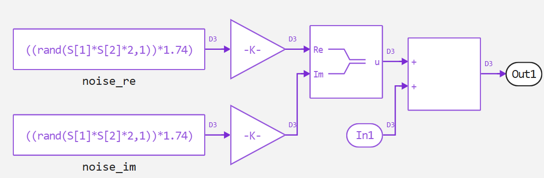
AGC is a system that automatically adjusts the signal gain level on the receiving side to maintain a constant output signal level regardless of changes in the input signal level. In our case, we have implemented logic that calculates the output power relative to the data before the signal is amplified, but you can easily replace this approach with a preset value.
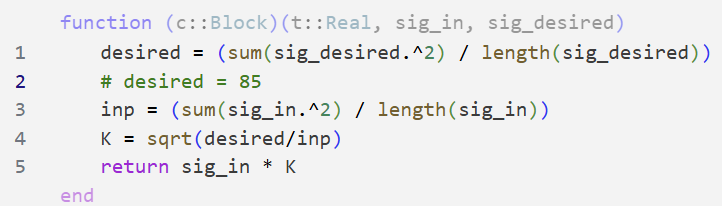
Based on the test below, we can clearly conclude that at 16-FSK, the desired signal power is 85 watts.
norm_img = ((channelview(inp_img))[:])
power_img = sum(norm_img.^2) / length(norm_img)
println("Input signal power: ", power_img, " Tue")

values = [1:2:15; -1:-2:-15]
v = [values[rand(1:length(values))] for _ in 1:length(norm_img)]
power_desired = sum(v .^ 2) / length(v)
println("Desired power: ", power_desired, " Tue")

K = sqrt(power_desired / power_img) # We use the square root, since the power is proportional to the square of the amplitude.
println("Gain factor: ", K)

amplified = norm_img .* K  # Enhanced signal

power_out = sum(amplified .^ 2) / length(amplified)
println("Output signal power: ", round(power_out, digits=2), " Tue")
The following blocks that we will consider are FM Modulator Baseband and FM Demodulator Baseband. This is a modulation that converts the base signal into a frequency-modulated (FM) signal.
Two key parameters are used in FM radio broadcasting.
-
The carrier frequency is the main frequency of the signal, which is modulated to transmit information. In the FM broadcasting range, it is between 87.5 MHz and 108 MHz.
-
The frequency of deviation is the maximum frequency deviation from the carrier frequency during signal transmission. For standard FM broadcasting, the maximum allowable deviation is ± 75 kHz.
Thus, if the carrier frequency is, say, 100 MHz, then the actual frequency of the transmitted signal will range from 99.925 to 100.075 MHz.
fs = 100e3 # Hz
println("Carrier frequency: $fs Hz")

deviation_fs = fs * 0.05 # 5% of fs
println("Frequency of deviation: $deviation_fs Hz")
The last block that we will consider is the communication channel block. To apply noise, it uses the Signal-to-Noise Ratio (SNR) metric, the signal-to-noise ratio. This metric shows how much stronger the useful signal is than the noise.
.png)
The higher the SNR, the higher the signal quality, as noise has less effect on the data. Conversely, the lower the SNR, the lower the signal quality, because noise begins to dominate the useful signal.
For example:
- If SNR = 20 dB, it means that the signal is 100 times more powerful than the noise (on a linear scale);
- If SNR = 0 dB, it means that the signal and noise power are equal;
- If SNR = -10 dB, it means that the noise is 10 times stronger than the signal.
snr = 10;
println("SNR: $snr dB")
snr_linear = 10^(snr / 10)
signal_power = 1
noise_power = 1 / snr_linear
println("Noise power: $noise_power")
Launching the model and analyzing the results
Let's set the simulation parameters and run the model.
st = 1/fs*S[1]*S[2] # Sample time
println("Time of one countdown: $st")
solver_step = st/S[1]/S[2]
println("Solver step: $solver_step")
time_stop = st*2.1
println("Simulation step: $st")
name_model = "SSTV"
Path = (@__DIR__) * "/" * name_model * ".engee"

if name_model in [m.name for m in engee.get_all_models()] # Checking the condition for loading a model into the kernel
    model = engee.open( name_model ) # Open the model
    model_output = engee.run( model, verbose=true ); # Launch the model
else
    model = engee.load( Path, force=true ) # Upload a model
    model_output = engee.run( model, verbose=true ); # Launch the model
    engee.close( name_model, force=true ); # Close the model
end
sleep(1)
Let's visualize the results of our model and summarize the results.
println("SNR: $snr dB")
println()
ber = ((collect(BER)).value)[end]
println("Total bits: $(Int(ber[3]))")
println("Number of errors: $(Int(ber[2]))")
println("BER: $(round(ber[1], digits=2))")

inp = plot(framestyle=:none, grid=false, title = "Entrance")
heatmap!( 1:S[2], 1:S[1], permutedims(inp_img, (2, 1)), colorbar=false)

sim_img = imrotate(colorview(Gray, ((collect(img_FM))[3,:].value)), deg2rad(-90))
sim = plot(framestyle=:none, grid=false, title = "Exit")
heatmap!( 1:size(sim_img, 2), 1:size(sim_img, 1), permutedims(sim_img, (2, 1)), colorbar=false)

sim_error = (collect(error_sim)).value
Average_error = round(sum(abs.(sim_error))/length(sim_error)*100, digits=2)
err = plot(sim_error, title = "The average error is $Average_error % ")

plot(plot(inp, sim), err, layout = grid(2, 1, heights=[0.7, 0.3]), legend=false)
As can be seen from the simulation results, we get good BER values at the output. If we take a closer look at the interleaving and scrambling settings, we can get an even better picture quality. For these purposes, you are provided with a second script SSTV_test. There is no superfluous description in it, but only the code of this project is given.
Conclusion
In this example, we examined the modeling capabilities of the slow-scan television-based image transmission protocol in Engee, and also explored many tools that allow us to perform such projects in Engee. As you can see from our example, Engee has all the necessary functions and tools for these models, and they work correctly.