Modulation analysis
In this example, we will analyze the possibilities of constructing constellations of various modulations.
The implemented demo model is shown below.
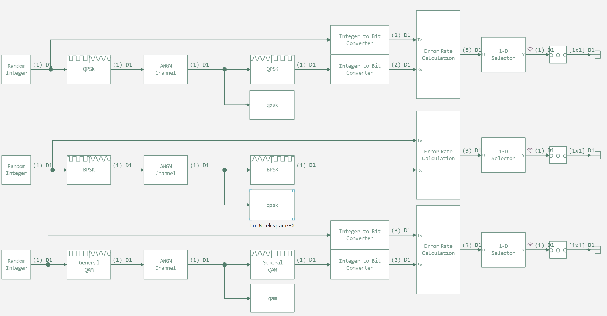
As we can see, there are 3 types of modulations used in this example.
- Quadrature phase keying (QPSK – quadrature phase-shift keying, or 4-PSK) uses a constellation of four points placed at equal distances on a circle.
- Binary phase keying (BPSK). With this modulation, two phase shifts are used (one for the logical unit and the second for the logical zero).
- Quadrature Amplitude Modulation (QAM) is a type of amplitude modulation of a signal, which is the sum of two carrier oscillations of the same frequency, but shifted in phase relative to each other by 90 ° (π/2 radians).
To begin with, we will declare the ratio of the energy of information bits per symbol to the spectral power density of noise.
Eb_No = 10;
Now let's declare the model launch function and run the simulation.
function run_model(name_model)
    Path = string(@__DIR__) * "/" * name_model * ".engee"

    if name_model in [m.name for m in engee.get_all_models()] # Checking the condition for loading a model into the kernel
        model = engee.open( name_model ) # Open the model
        model_output = engee.run( model, verbose=true ); # Launch the model
    else
        model = engee.load( Path, force=true ) # Upload a model
        model_output = engee.run( model, verbose=true ); # Launch the model
        engee.close( name_model, force=true ); # Close the model
    end
    return model_output
end
run_model("demo_model")
Let's perform the construction of a guide for each of the modulations. Let's start with QPSK, and then build BPSK and 8-PSK.
qpsk = collect(qpsk);
qpsk_new = [(i...)+0 for i in qpsk.value];
plot(title="QPSK")
plot!(ComplexF64.(qpsk_new), seriestype=:scatter)
plot!([0.75+0.75im, 0.75-0.75im, -0.75+0.75im, -0.75-0.75im], seriestype=:scatter)
bpsk = collect(bpsk);
bpsk_new = [(i...)+0 for i in bpsk.value];
plot(title="BPSK")
plot!(ComplexF64.(bpsk_new), seriestype=:scatter)
plot!([-1+0im, 1+0im], seriestype=:scatter)
qam = collect(qam);
qam_new = [(i...)+0 for i in qam.value];
plot(title="8-PSK")
plot!(ComplexF64.(qam_new), seriestype=:scatter)
plot!(cis.(2pi*[0:7...]/8), seriestype=:scatter)
As we can see from the above constellations, the first two modulations have a more pronounced point spacing. And in the first two variants, there are significantly fewer areas of intersection of points, which is why we got four times less bit error values in QPSK and BPSK than when using 8-PSK.
Conclusion
In this example, we have considered ways to construct and analyze modulated signals using the example of QPSK, BPSK and QAM modulations.