Digital communication channel
In this example, we demonstrate a block chain for creating a digital communication channel. The model implements a modulator, receiving and transmitting filters for Manchester encoding, a channel with white noise, signal decoding and error counting.
The example uses Engee's ability to work with models in which different simulation rates are set for individual subsystems. In this model, there are subsystems operating at different frequencies.:
- 2.5 Hz – frequency at the “application level” of the model (the generator generates numbers from 0 to 10)
- 10 Hz – frequency of the bit stream after digital modulation (4-bit packets)
- 80 Hz – frequency at the physical level (bipolar digital signal and the Manchester encoding is 1 to 8)
Errors are calculated on the receiving side, both at the number level and at the bit level.
The structure of the model
The model includes:
- Generator of numbers from 0 to 10
- A modulator that translates them into 4-bit sequences
- Converter of a unipolar signal to a bipolar one
- Digital filter for application to the Manchester code signal
- Channel with added Gaussian noise
And a set of reverse operations:
- Paired receiving filter for the Manchester code
- Converter from bipolar signal to unipolar
- Bit error counting unit between the sent and received signal
- Demodulator, which makes numbers from 0 to 10 from each group of 4 bits.
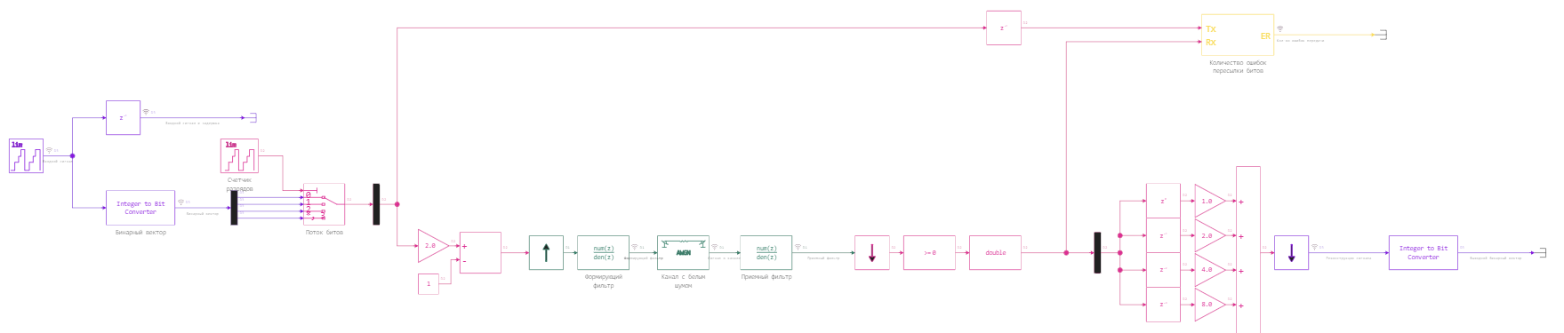
General view of the model
.png)
This model allows you to look into each communication line and see what the signal is at each stage of transmission.
Launching a model from a script
To automate the analysis, you need to close the model (if it is open on the canvas) and run this model under program control.
Pkg.add(["Measures"])
# Launching the model
model = engee.open("$(@__DIR__)/simple_digital_channel.engee");
results = engee.run( model )
# engee.close( "simple_digital_channel", force=true );
Conclusion of graphs
Connecting libraries
# Connecting libraries
using DataFrames, Measures
gr(); # Enabling a backend graphics display method
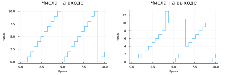
Analysis of input and output information (a series of numbers)
# Uploading data
Sin = results["Input signal and delay"];
Sout = results["Signal reconstruction"];

# Plotting graphs
plot(
    plot( Sin.time, Sin.value, st=:step, xlabel="Time", ylabel="Numbers", title="The numbers in the input", leg=false ),
    plot( Sout.time, Sout.value, st=:step, xlabel="Time", ylabel="Numbers", title="The numbers in the output", leg=false ),
    layout=grid(1, 2, widths=(4/8,4/8)), size=(900,300), margin=5mm, guidefont = font( 7 )
)
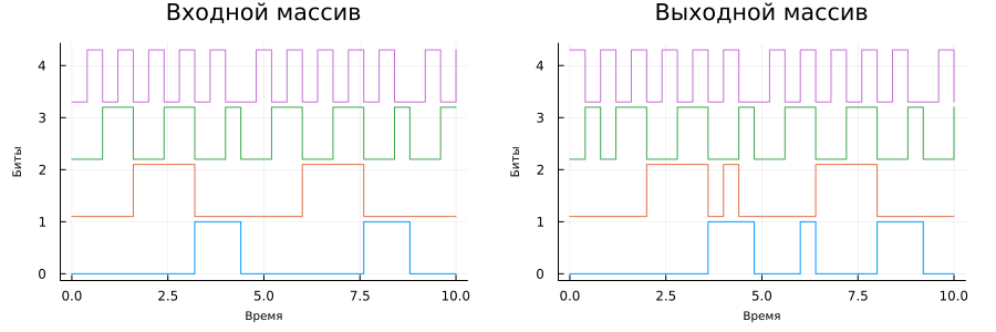
Analysis of input and output bit arrays
# Uploading data
Bin = results["Binary vector"]
Bout = results["The output binary vector"]

Bin_a = [v[1] for v in Bin.value]
Bin_b = [v[2] for v in Bin.value]
Bin_c = [v[3] for v in Bin.value]
Bin_d = [v[4] for v in Bin.value]

Bout_a = [v[1] for v in Bout.value]
Bout_b = [v[2] for v in Bout.value]
Bout_c = [v[3] for v in Bout.value]
Bout_d = [v[4] for v in Bout.value]

# Plotting graphs
plot(
    plot( Bin.time, [Bin_a Bin_b.+1.1 Bin_c.+2.2 Bin_d.+3.3], st=:step,
      xlabel="Time", ylabel="Bits", title="The input array", leg=false ),
    plot( Bout.time, [Bout_a Bout_b.+1.1 Bout_c.+2.2 Bout_d.+3.3], st=:step,
      xlabel="Time", ylabel="Bits", title="Output array", leg=false ),
    layout=grid(1, 2, widths=(4/8,4/8)), size=(900,300), margin=5mm, guidefont = font( 7 )
)
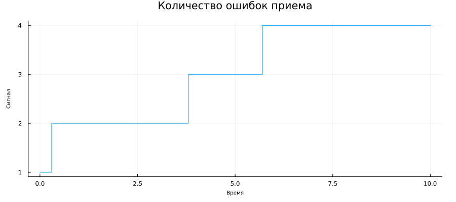
Let's display the number of mistakenly received bits.
# Uploading data
ERC = results["Number of transmission errors"]

# Plotting graphs
plot(
    plot( ERC.time, ERC.value, st=:step, xlabel="Time", ylabel="The signal", title="Number of reception errors", leg=false ),
    size=(900,400), margin=5mm, guidefont = font( 7 )
)
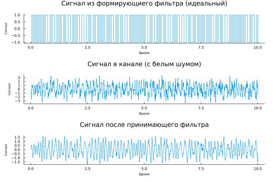
Let's study the noise in the channel
# Uploading data
Fin = results["Forming Filter"];
AWGN_out = results["The signal in the channel"];
Fout = results["Receiving filter"];

# Plotting graphs
plot(
    plot( Fin.time, Fin.value, st=:step, xlabel="Time", ylabel="The signal", title="Signal from the forming filter (ideal)", leg=false ),
    plot( AWGN_out.time, AWGN_out.value, st=:step, xlabel="Time", ylabel="The signal", title="Channel signal (with white noise)", leg=false ),
    plot( Fout.time, Fout.value, st=:step, xlabel="Time", ylabel="The signal", title="The signal after the receiving filter", leg=false ),
    layout=grid(3, 1),
    size=(900,600), margin=5mm, guidefont = font( 7 )
)
Conclusion
Based on this example, you can calculate coding redundancy parameters, check error correction codes, or check the operation of a communication channel at the physical level with other signal encoding: frequency, phase, make the channel part of a virtual booth, and much more.
The Engee platform allows you to demonstrate the work of digital electronics very clearly, select parameters and debug algorithms, and back up everything with visual illustrations.