QPSK and the effects of time synchronization
In modern digital communication systems, ensuring high reliability of information transmission in the presence of interference and limited channel bandwidth remains a critical task. One of the key modulation schemes widely used in various wireless communication standards is quadrature phase shift keying (QPSK), which ensures efficient use of the spectrum by transmitting two bits of information per symbol.
This paper presents a comprehensive model of a communication system with QPSK modulation, developed to study the effect of sampling timing on the noise immunity of the system. The model includes a complete signal transmission path: from random data generation and modulation to the demodulation process under conditions of additive white Gaussian noise (AWGN).
A key feature of this implementation is the study of the effect of the time synchronization parameter (Select_index) on the probability of a bit error (BER). The raised cosine filter of the transmitter increases the number of samples from 1 to 8 per symbol, while the receiver filter retains this increased number of samples. The function of the selector is to select one of the eight possible sampling points for subsequent demodulation.
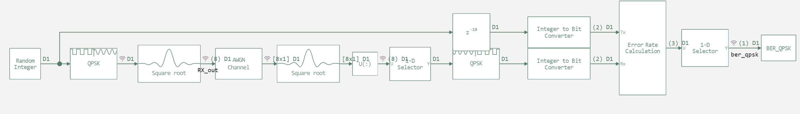
The model implements the following key stages of signal processing:
- Generating random integer data and converting it to QPSK characters
- The raised cosine filtering stage (8 counts per character)
- Adding Gaussian noise with a given Eb/No ratio
- Consistent filtering of the received signal while maintaining over-sampling
- Selection of the optimal sampling moment via the Select_index parameter (1-8)
- QPSK demodulation and calculation of the bit error probability
Now let's run our model with the initial parameters using the model startup function and see the BER results.
The code below implements the function run_model() to manage the launch of the model in the Engee environment. The function performs:
- Checking for an already loaded model in the kernel
- If not present, loads the model from a file with the extension
.engee - Runs the model with the output of the progress of execution
- Automatically closes the model after execution
function run_model(name_model)
    Path = string(@__DIR__) * "/" * name_model * ".engee"

    if name_model in [m.name for m in engee.get_all_models()] # Checking the condition for loading a model into the kernel
        model = engee.open( name_model ) # Open the model
        model_output = engee.run( model, verbose=true ); # Launch the model
    else
        model = engee.load( Path, force=true ) # Upload a model
        model_output = engee.run( model, verbose=true ); # Launch the model
        engee.close( name_model, force=true ); # Close the model
    end
    return model_output
end
Key parameters:
Eb_No = 13- signal-to-noise ratio per bit (13 dB)Select_index = 1- index of the sampling moment selection
Eb_No = 13;
Select_index = 1;

run_model("QPSK_timing_sync"); # Launching the model.
println(simout)
println()
println("BER: $(collect(BER_QPSK).value[end][1])")
Execution results:
- The model is being compiled successfully with step-by-step progress
- The structure is displayed
SimulationResultwith output signals:RX_out- the received signal after the receiver filterВыбор.1- selected counts for demodulationber_qpsk- calculated probability of a bit error
- The calculated BER value is 0.0065 (0.65%) for the specified conditions
The obtained BER value demonstrates good communication quality at the selected Eb/No ratio and the first sampling moment.
Next, we will analyze the energy spectrum of the QPSK signal, the code below performs the calculation and visualization of the energy spectrum of the signal after the filter of the transmitter with an elevated cosine.
Key processing steps:
-
Signal extraction - receives a complex signal after the transmission filter
-
Calculation of the spectral power density:
- Calculation of the FFT signal
- Normalization to signal length and sampling frequency (800 Hz)
- Conversion to a logarithmic scale (dB)
-
Smoothing the spectrum:
- Application of a moving average with a window of 20 counts
- Elimination of edge effects of convolution
-
Plotting:
- Centering the frequency axis relative to zero
- Display in the range ±400 Hz (half the sampling frequency)
# Connecting libraries
neededLibs = ["FFTW", "DSP", "Statistics"]
for lib in neededLibs
    try
        eval(Meta.parse("using $lib"))
    catch ex
        Pkg.add(lib)
        eval(Meta.parse("using $lib"))
    end
end
Out_Transmit_Filter_value = vcat(simout["QPSK_timing_sync/RX_out"].value...)
fs = 800
power_spectrum_raw = abs.(fft(Out_Transmit_Filter_value)).^2 / (length(Out_Transmit_Filter_value) * fs)
power_spectrum_db_raw = 10*log10.(power_spectrum_raw)
window_size = 20
kernel = ones(window_size) / window_size
power_spectrum_smoothed = conv(power_spectrum_db_raw, kernel)[window_size÷2+1:end-window_size÷2]
freqs = fftfreq(length(power_spectrum_smoothed), fs)

plot(fftshift(freqs), fftshift(power_spectrum_smoothed),
     title="Energy spectrum (moving average, window $window_size)",
     xlabel="Frequency, Hz",
     ylabel="Spectral power density, dB/Hz",
     legend=false,
     linewidth=2,
     grid=true)
The graph shows an almost perfectly formed spectrum of the QPSK signal with the characteristics:
- Flat top in the bandwidth (except for 0)
- Steep attenuation slopes outside the baseband
- Minimal out-of-band emissions are the result of efficient operation of the raised cosine filter
- Symmetrical shape relative to zero frequency
The spectrum demonstrates excellent spectral characteristics of the system, which confirms the correct operation of the transmitter filter and efficient use of the frequency band.
Next, we proceed to testing with different values for Select_index.
ber_qpsk = zeros(8);
RX_out = Vector{Vector{ComplexF64}}(undef, 8)
Selection_data = Vector{Vector{ComplexF64}}(undef, 8)
fs = 800
global Select_index

@time for i in 1:8
    println("Running the model for Select_index = $i")
    Select_index = Int32(i)
    run_model("QPSK_timing_sync")
    ber_qpsk[i] = collect(BER_QPSK).value[end][1]
    RX_out[i] = vcat(simout["QPSK_timing_sync/RX_out"].value...)
    Selection_data[i] = simout["QPSK_timing_sync/Choice.1"].value
end
Collected data:
- BER values for 8 different sampling points
- Receiver output signals (RX_out) for each case
- Selected samples (Selection_data) for time synchronization analysis
The test has been successfully completed and is ready for further analysis of the dependence of BER on the choice of sampling moment, which is critically important for assessing the impact of time synchronization on the quality of communication in the QPSK system.
println("\Presults BER:")
for i in 1:8
    println("Select_index = $i: BER = $(ber_qpsk[i])")
end
plot(1:8, ber_qpsk,
     title="BER's dependence on Select_index",
     xlabel="Select_index",
     ylabel="BER",
     marker=:circle,
     linewidth=2,
     grid=true,
     legend=false,
     yscale=:log10)
Analysis of the dependence of BER on the sampling moment
The graph on a logarithmic scale clearly demonstrates the exponential nature of the degradation of communication quality when deviating from the optimal sampling moment. Optimal sampling times: Select_index = 2: BER = 0.0060 (best result) and Select_index = 1 BER = 0.0065 (very close to optimal). Critical quality degradation begins with Select_index = 3 BER = 0.0135 (2 times worse than optimal), and the worst cases are Select_index = 5-8: BER > 0.25 (actually loss of connection)
Based on this, the following conclusions can be drawn:
- Optimal synchronization is achieved at indexes 1 and 2
- Sharp degradation begins with index 3
- Zero efficiency at indexes 5-8 (BER ≈ 0.5 - equivalent to random guessing)
Next, let's take a closer look at the best and worst results.
best_idx = argmin(ber_qpsk)
worst_idx = argmax(ber_qpsk)
best_selection = Selection_data[best_idx]
worst_selection = Selection_data[worst_idx]
downsample_factor = 20
best_constellation = best_selection[1:downsample_factor:end]
worst_constellation = worst_selection[1:downsample_factor:end]
function compute_spectrum_q(signal, fs)
    q_signal = imag(signal)
    N = length(q_signal)
    power_spectrum = abs.(fft(q_signal)).^2 / (N * fs)
    power_spectrum_db = 10*log10.(power_spectrum)
    freqs = fftfreq(N, fs)
    return fftshift(freqs), fftshift(power_spectrum_db)
end
freqs_best, spectrum_best = compute_spectrum_q(RX_out[best_idx], fs)
freqs_worst, spectrum_worst = compute_spectrum_q(RX_out[worst_idx], fs)
p_combined = plot(layout=(3,1), size=(800, 900))

t = 1:200
plot!(p_combined[1], t, imag(best_selection[t]),
      label="The best (Index $best_idx)", linewidth=2, color=:blue)
plot!(p_combined[1], t, imag(worst_selection[t]),
      label="The worst (Index $worst_idx)", linewidth=2, color=:red, linestyle=:dash)
title!(p_combined[1], "Temporary data of the Q component")

plot!(p_combined[2], freqs_best, spectrum_best,
      label="The best", linewidth=2, color=:blue)
plot!(p_combined[2], freqs_worst, spectrum_worst,
      label="Worse", linewidth=2, color=:red, linestyle=:dash)
title!(p_combined[2], "Spectra of Q components")

scatter!(p_combined[3], 1:length(best_constellation), imag(best_constellation),
         label="The best", markersize=4, alpha=0.7, color=:blue,
         markerstrokewidth=0, marker=:circle)
scatter!(p_combined[3], 1:length(worst_constellation), imag(worst_constellation),
         label="Worse", markersize=4, alpha=0.7, color=:red,
         markerstrokewidth=0, marker=:x)
title!(p_combined[3], "Q components of constellations")
plot!(p_combined, titlefontsize=12, legendfontsize=10)
These graphs show the following:
- The spectra are identical → Filtering works equally well in both cases
- The time data is different → The sampling moment is critically important
- Constellations are different → Optimal synchronization (blue dots) gives clear clusters, poor synchronization (red crosses) - blurred
From this we can conclude that the problem is not in filtering or signal quality, but solely in the accuracy of time synchronization. The system requires precise sampling timing for correct demodulation.
Conclusion
The conducted study demonstrates a significant dependence of BER on the choice of sampling moment, which confirms the critical importance of accurate time synchronization in real digital communication systems. The results show that only the first three sampling moments provide acceptable communication quality, while the choice of subsequent moments leads to a sharp deterioration in system performance.