Calculation of BER for 8-PSK
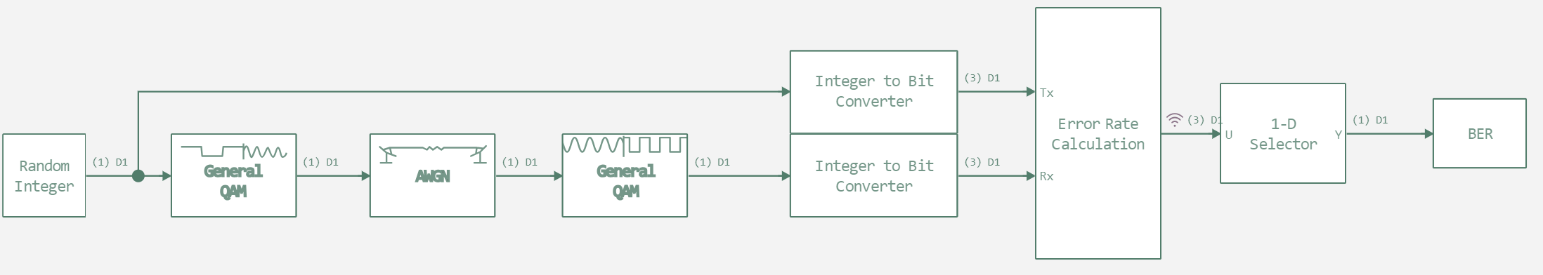
The Error Rate Calculation block calculates the error rate by bits (bit error rate, BER). Using this block, we can obtain BER data for the communication system and analyze the effectiveness of our system. In this example, we will look at a simple 8-PSK receiver and transmitter model. It is shown in the picture below.
Next, we will set an auxiliary function to run the model.
# Enabling the auxiliary model launch function.
function run_model( name_model)

    Path = (@__DIR__) * "/" * name_model * ".engee"

    if name_model in [m.name for m in engee.get_all_models()] # Checking the condition for loading a model into the kernel
        model = engee.open( name_model ) # Open the model
        model_output = engee.run( model, verbose=true ); # Launch the model
    else
        model = engee.load( Path, force=true ) # Upload a model
        model_output = engee.run( model, verbose=true ); # Launch the model
        engee.close( name_model, force=true ); # Close the model
    end
    sleep(0.5)
    return model_output
end
Next, we will initialize the signal-to-noise ratio indicators for our model and declare a bit error variable.
EbNoArr = collect(-9:3:9);
Eb_No = 0;
ber = zeros(length(EbNoArr));
BER = 0;
Now let's run the model at different values of the signal-to-noise ratio.
for i in 1:length(EbNoArr)
    Eb_No = EbNoArr[i]
    run_model("8-PSK") # Launching the model.
    BER = collect(BER)
    ber[i]=BER.value[end][1]
    println("BER: $(ber[i])")
end
We will construct a BER graph from both the model and theoretical calculations.
using SpecialFunctions
function berawgn_psk(EbNo_dB, M)
    EbNo = 10 .^ (EbNo_dB ./ 10)
    k = log2(M)
    # The coefficient α depends on Eb/No: ~1.5-1.7
    α = 1.6 # the average value
    return α * erfc.(sqrt.(k * EbNo) * sin(π / M)) / k
end
ber_ref = berawgn_psk(EbNoArr, 8)
println("__Eb_No__: $EbNoArr")
println("_ber_ref_: $(round.(ber_ref, digits=3))")
println("ber_model: $(round.(ber, digits=3))")

p1 = plot(EbNoArr, ber_ref, seriestype = :scatter, marker = :rect, label = "Theoretical QPSK", yscale = :log10)
plot!(p1, EbNoArr, ber, seriestype = :scatter, marker = :diamond, label = "Model QPSK")
xlabel!(p1, "Eb/No (dB)")
ylabel!(p1, "BER")
title!(p1, "Bit Error Rate (Log Scale)")
# Second graph: normal scale
p2 = plot(EbNoArr, ber_ref, seriestype = :scatter, marker = :rect, label = "")
plot!(p2, EbNoArr, ber, seriestype = :scatter, marker = :diamond, label = "")
ylabel!(p2, "BER")
title!(p2, "Bit Error Rate (Linear Scale)")

# The general conclusion: two graphs side by side
plot(p2, p1, layout = (2, 1), size=(1000,400))
Conclusion
As you can see in this example, the higher the signal-to-noise ratio, the lower the error.
Here we have figured out how to build a BER graph for a simple communication system model and learned how to apply this method to analyze the system.