数据读取器
|
该页面正在翻译中。 |
#
<无翻译>*麦琪数据读取器*-Function
datashader(points::AbstractVector{<: Point})|
警告此功能可能会在中断版本之外更改,因为API尚未最终确定。 如果您遇到奇怪的行为,请警惕实现中的错误和开放的问题。 |
点可以是任何支持迭代和getindex的数组类型,包括内存映射数组。 如果您有x和y坐标的单独数组,并且希望避免转换和复制,请考虑使用:
using Makie.StructArrays
points = StructArray{Point2f}((x, y))
datashader(points)
请注意,如果x和y没有实现快速迭代/getindex,这可能比将数据复制到新数组中要慢。
为了获得最佳性能,请使用 方法=Makie。攻击线程() 一定要从茱莉亚开始 茱莉亚-陶托 或者有环境变量 JULIA_NUM_线程 设置为您拥有的内核数。
地块类型
绘图类型别名 数据读取器 功能是 数据读取器.
例子:
机场
using GLMakie
using DelimitedFiles

airports = Point2f.(eachrow(readdlm(assetpath("airportlocations.csv"))))
fig, ax, ds = datashader(airports,
    colormap=[:white, :black],
    # for documentation output we shouldn't calculate the image async,
    # since it won't wait for the render to finish and inline a blank image
    async = false,
    figure = (; figure_padding=0, size=(360*2, 160*2))
)
Colorbar(fig[1, 2], ds, label="Number of airports")
hidedecorations!(ax); hidespines!(ax)
fig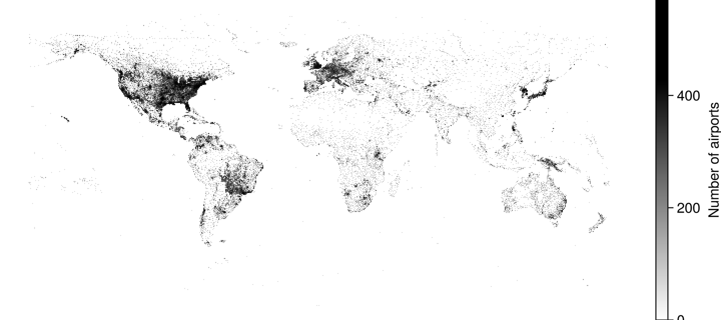
均值聚合
using GLMakie
with_z(p2) = Point3f(p2..., cos(p2[1]) * sin(p2[2]))
points = randn(Point2f, 100_000)
points_with_z = map(with_z, points)

f = Figure()
ax = Axis(f[1, 1], title = "AggMean")
datashader!(ax, points_with_z, agg = Makie.AggMean(), operation = identity)
ax2 = Axis(f[1, 2], title = "AggMean binsize = 3")
datashader!(ax2, points_with_z, agg = Makie.AggMean(), operation = identity, binsize = 3)
f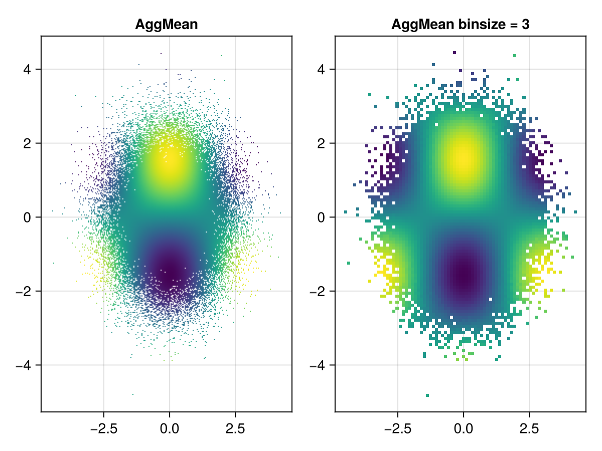
奇怪的吸引子
using GLMakie
# Taken from Lazaro Alonso in Beautiful Makie:
# https://beautiful.makie.org/dev/examples/generated/2d/datavis/strange_attractors/?h=cliffo#trajectory
Clifford((x, y), a, b, c, d) = Point2f(sin(a * y) + c * cos(a * x), sin(b * x) + d * cos(b * y))

function trajectory(fn, x0, y0, kargs...; n=1000) #  kargs = a, b, c, d
    xy = zeros(Point2f, n + 1)
    xy[1] = Point2f(x0, y0)
    @inbounds for i in 1:n
        xy[i+1] = fn(xy[i], kargs...)
    end
    return xy
end

cargs = [[0, 0, -1.3, -1.3, -1.8, -1.9],
    [0, 0, -1.4, 1.6, 1.0, 0.7],
    [0, 0, 1.7, 1.7, 0.6, 1.2],
    [0, 0, 1.7, 0.7, 1.4, 2.0],
    [0, 0, -1.7, 1.8, -1.9, -0.4],
    [0, 0, 1.1, -1.32, -1.03, 1.54],
    [0, 0, 0.77, 1.99, -1.31, -1.45],
    [0, 0, -1.9, -1.9, -1.9, -1.0],
    [0, 0, 0.75, 1.34, -1.93, 1.0],
    [0, 0, -1.32, -1.65, 0.74, 1.81],
    [0, 0, -1.6, 1.6, 0.7, -1.0],
    [0, 0, -1.7, 1.5, -0.5, 0.7]
]

fig = Figure(size=(1000, 1000))
fig_grid = CartesianIndices((3, 4))
cmap = to_colormap(:BuPu_9)
cmap[1] = RGBAf(1, 1, 1, 1) # make sure background is white

let
    # locally, one can go pretty high with n_points,
    # e.g. 4*(10^7), but we don't want the docbuild to become too slow.
    n_points = 10^6
    for (i, arg) in enumerate(cargs)
        points = trajectory(Clifford, arg...; n=n_points)
        r, c = Tuple(fig_grid[i])
        ax, plot = datashader(fig[r, c], points;
            colormap=cmap,
            async=false,
            axis=(; title=join(string.(arg), ", ")))
        hidedecorations!(ax)
        hidespines!(ax)
    end
end
rowgap!(fig.layout,5)
colgap!(fig.layout,1)
fig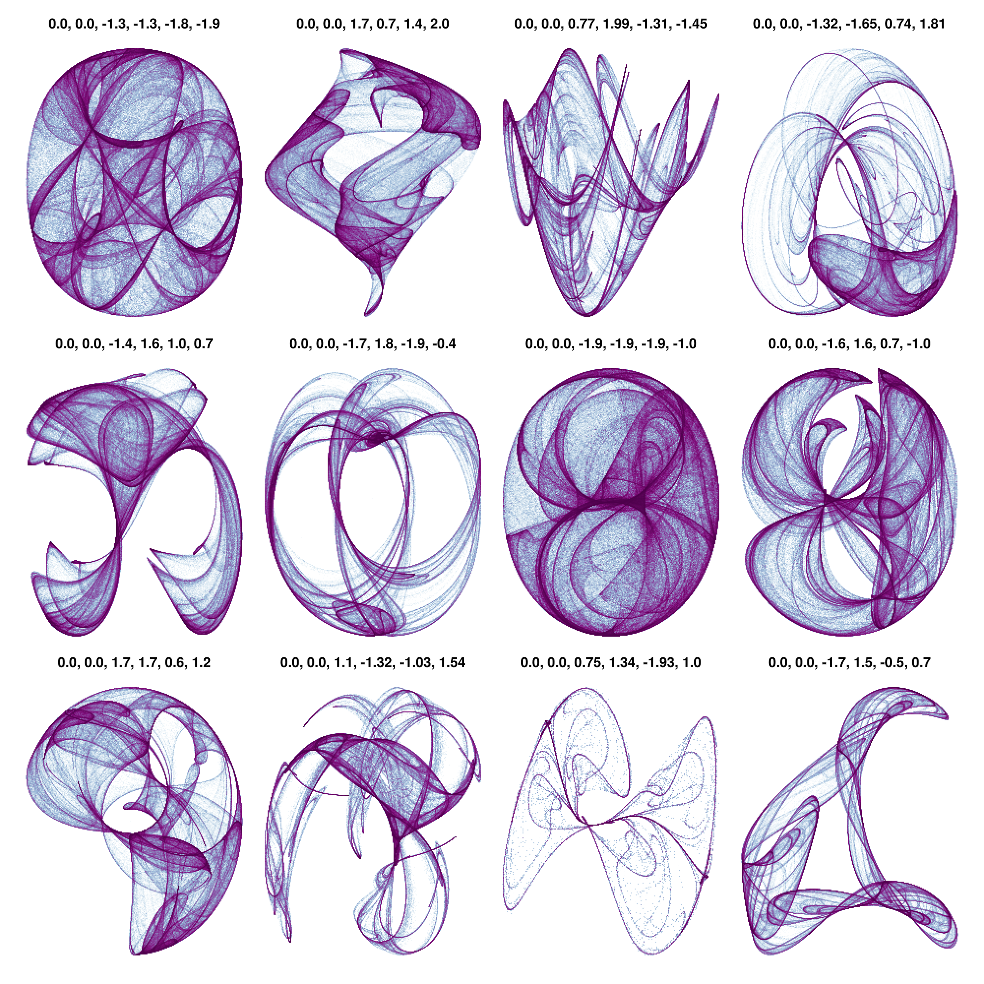
更大的例子
评论中的时间来自在32gb Ryzen5800h笔记本电脑上运行此操作。 这两个例子还没有完全优化,只是使用原始的,未排序的,内存映射的Point2f数组。 将来,我们需要添加加速结构来优化对子区域的访问。
1400万点纽约出租车数据集
using GLMakie, Downloads, Parquet2
bucket = "https://ursa-labs-taxi-data.s3.us-east-2.amazonaws.com"
year = 2009
month = "01"
filename = join([year, month, "data.parquet"], "/")
out = joinpath("$year-$month-data.parquet")
url = bucket * "/" * filename
Downloads.download(url, out)
# Loading ~1.5s
@time begin
    ds = Parquet2.Dataset(out)
    dlat = Parquet2.load(ds, "dropoff_latitude")
    dlon = Parquet2.load(ds, "dropoff_longitude")
    # One could use struct array here, but dlon/dlat are
    # a custom array type from Parquet2 supporting missing and some other things, which slows the whole thing down.
    # points = StructArray{Point2f}((dlon, dlat))
    points = Point2f.(dlon, dlat)
    groups = Parquet2.load(ds, "vendor_id")
end

# ~0.06s
@time begin
    f, ax, dsplot = datashader(points;
        colormap=:fire,
        axis=(; type=Axis, autolimitaspect = 1),
        figure=(;figure_padding=0, size=(1200, 600))
    )
    # Zoom into the hotspot
    limits!(ax, Rect2f(-74.175, 40.619, 0.5, 0.25))
    # make image fill the whole screen
    hidedecorations!(ax)
    hidespines!(ax)
    display(f)
end27亿OSM GPS点
下载数据从https://planet.osm.org/gps/simple-gps-points-120604.csv.xz[OSM GPS点]并使用https://gist.github.com/SimonDanisch/69788fce47c13020d9ae9dbe08546f89#file-datashader-2-7-billion-points-jl[更新的脚本]从https://medium.com/hackernoon/drawing-2-7-billion-points-in-10s-ecc8c85ca8fa[drawing-2-7-billion-points-in-10s]将CSV转换为我们可以记忆映射的二进制blob。
using GLMakie, Mmap
path = "gpspoints.bin"

points = Mmap.mmap(open(path, "r"), Vector{Point2f});
# ~ 26s
@time begin
    f, ax, pl = datashader(
        points;
        # For a big dataset its interesting to see how long each aggregation takes
        show_timings = true,
        # Use a local operation which is faster to calculate and looks good!
        local_operation=x-> log10(x + 1),
        #=
            in the code we used to save the binary, we had the points in the wrong order.
            A good chance to demonstrate the `point_transform` argument,
            Which gets applied to every point before aggregating it
        =#
        point_transform=reverse,
        axis=(; type=Axis, autolimitaspect = 1),
        figure=(;figure_padding=0, size=(1200, 600))
    )
    hidedecorations!(ax)
    hidespines!(ax)
    display(f)
end
aggregation took 1.395s aggregation took 1.176s aggregation took 0.81s aggregation took 0.791s aggregation took 0.729s aggregation took 1.272s aggregation took 1.117s aggregation took 0.866s aggregation took 0.724s
分类数据
现在有两种方法可以绘制分类数据:
datashader(one_category_per_point, points)
datashader(Dict(:category_a => all_points_a, :category_b => all_points_b))using GLMakie
normaldist = randn(Point2f, 1_000_000)
ds1 = normaldist .+ (Point2f(-1, 0),)
ds2 = normaldist .+ (Point2f(1, 0),)
fig, ax, pl = datashader(Dict("a" => ds1, "b" => ds2); async = false)
hidedecorations!(ax)
fig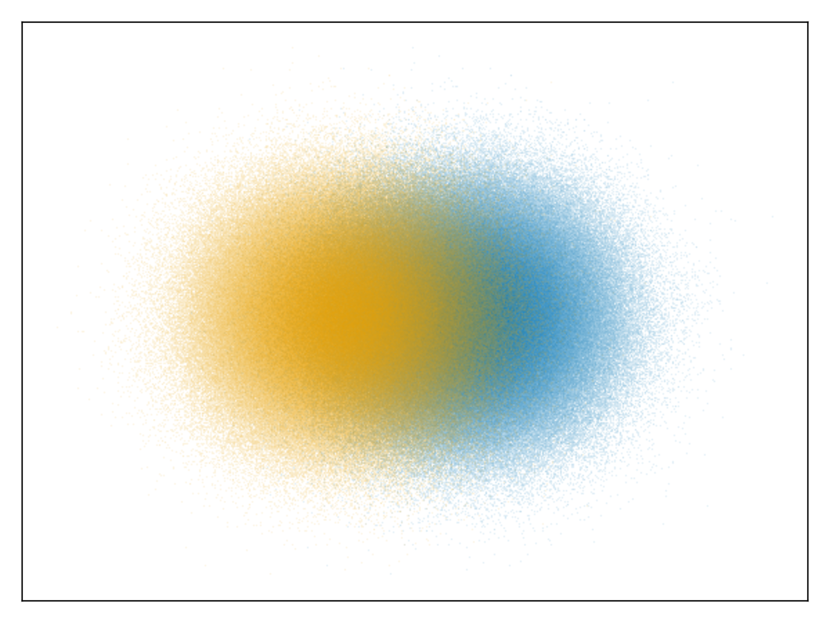
我们还可以将前面的NYC示例重复用于分类图:
@time begin
    f = Figure(figure_padding=0, size=(1200, 600))
    ax = Axis(
        f[1, 1],
        autolimitaspect=1,
        limits=(-74.022, -73.827, 40.696, 40.793),
        backgroundcolor=:black
    )
    datashader!(ax, groups, points)
    hidedecorations!(ax)
    hidespines!(ax)
    # Create a styled legend
    axislegend("Vendor ID"; titlecolor=:white, framecolor=:grey, polystrokewidth=2, polystrokecolor=(:white, 0.5), rowgap=10, backgroundcolor=:black, labelcolor=:white)
    display(f)
end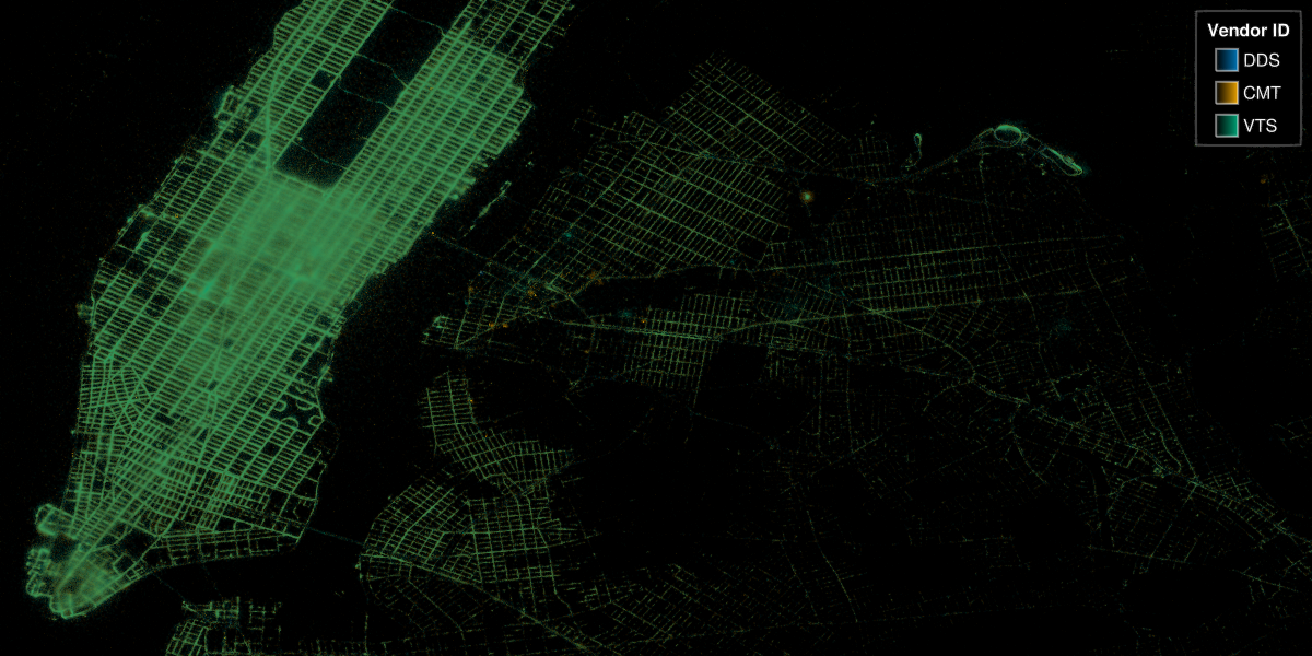
属性
署理主任
默认值为 AggCount{Float32}()
可以是 AggCount(), 阿加尼() 或 阿格米恩(). 确保使用正确的元素类型,例如 AggCount{Float32}(),其中需要容纳的输出 本地操作. 通过重载实现用户可扩展:
struct MyAgg{T} <: Makie.AggOp end
MyAgg() = MyAgg{Float64}()
Makie.Aggregation.null(::MyAgg{T}) where {T} = zero(T)
Makie.Aggregation.embed(::MyAgg{T}, x) where {T} = convert(T, x)
Makie.Aggregation.merge(::MyAgg{T}, x::T, y::T) where {T} = x + y
Makie.Aggregation.value(::MyAgg{T}, x::T) where {T} = x夹式飞机
默认值为 自动的
剪辑平面提供了一种在3D空间中进行剪辑的方法。 您可以设置最多8个向量 平面3f 飞机在这里,后面的情节将被裁剪(即变得不可见)。 默认情况下,剪辑平面继承自父绘图或场景。 您可以删除父 夹式飞机 通过传递 平面3f[].