bandstop
Signals after the notch filter.
| Library |
|
Syntax
Function call
-
y = bandstop(x,wpass)— filters the input signalxusing a notch filter with a delay band frequency range specified by a two-element vectorwpassin standardized units rad/countdown. Functionbandstopuses a minimum order filter with bandwidth attenuation60dB and compensates for the delay introduced by the filter. Ifx— matrix, the function filters each column independently.
-
y = bandstop(_, Name,Value)— sets additional options for any of the previous syntaxes with one or more argumentsName,Value.
-
y = bandstop(_; out=:plot)— Plots the input signal and overlays the filtered signal.
Arguments
Input arguments
# x — input signal
+
vector | the matrix
Details
An input signal specified as a vector or matrix.
| Data types |
|
| Support for complex numbers |
Yes |
#
wpass —
normalized frequency range
of the delay band
vector
Details
The normalized frequency range of the delay band, defined as a two-element vector with elements in the interval (0, 1).
#
fs —
sampling
rate
scalar
Details
The sampling frequency, set as a positive real scalar.
Name-value input arguments
Specify optional argument pairs in the format Name, Value, where Name — the name of the argument, and Value — the appropriate value. Name-value arguments should be placed after other arguments, but the order of the pairs does not matter.
Use commas to separate the name and value, and Name put it in quotation marks.
Example: f = bandstop(x, 200, fs, "StopbandAttenuation", 30).
# ImpulseResponse — type of impulse response
+
"auto" (by default) | "fir" | "iir"
Details
The type of pulse response of the filter, set as "fir", "iir" or "auto":
-
"fir"— the function designs a minimum-order filter, linear-phase, with a finite impulse response (FIR). To compensate for the delay, the function adds to the input signal zeros, where — filter order. The function then filters the signal and deletes the first ones. counts at the output.In this case, the input signal must be at least twice as long as the filter that meets the specifications.
-
"iir"— the function designs a minimum-order filter with infinite impulse response (BIH) and uses the functionfiltfiltto perform zero-phase filtering and filter delay compensation.If the signal is less than three times longer than the filter that meets the specification, the function designs a filter of a lower order and, therefore, a lower steepness.
-
"auto"— the function designs a minimum-order FIR filter if the input signal is long enough, and a minimum-order FIR filter otherwise. Specifically, the function performs the following steps:-
Calculates the minimum order that the FIR filter must have in order to meet the specifications. If the signal is at least twice as long as the required filter order, it designs and uses this filter.
-
If the signal is not long enough, calculates the minimum order that the FIR filter must have in order to meet the specifications. If the signal length is at least three times the required filter order, it designs and uses this filter.
-
If the signal length is insufficient, truncates the order to one-third of the signal length and designs an IIR filter of this order. The decrease in order occurs due to the steepness of the transition band decline.
-
Filters the signal and compensates for the delay.
-
# Steepness — steepness of the transition band decline
+
[0.85 0.85] (by default) | vector | scalar
Details
The slope of the transition band decline, defined as a two-element vector with elements in the interval [0.5, 1) or a scalar in the interval [0.5, 1). As the steepness increases, the impulse response of the filter approaches the ideal impulse response of the notch filter, but the resulting filter length also increases, as well as the computational cost of the filtration operation. For more information, see The steepness of the decline of the notch filter.
# StopbandAttenuation — attenuation in the delay band of the filter
+
60 (by default) | positive scalar
Details
The attenuation in the filter’s delay band, set as a positive scalar in dB.
Output arguments
# y — filtered signal
+
vector | the matrix
Details
The filtered signal returned as a vector or matrix with the same dimensions as the input signal.
Examples
Notch tone filtering
Details
We will generate a signal sampled with the frequency 1 kHz during 1 seconds. The signal contains three tones: with a frequency of 50 Hz, 150 Hz and 250 Hz. The amplitude of the high-frequency and low-frequency tones is twice the amplitude of the intermediate tone. Gaussian white noise with variance is added to the signal 1/100.
import EngeeDSP.Functions: bandstop, randn

fs = 1e3
t = 0:1/fs:1
x = [2 1 2] * sin.(2π * [50; 150; 250] .* reshape(t, 1, :)) + randn(1, length(t)) / 10
Filter the signal using a notch filter to remove the intermediate tone. Specify the frequency of the delay band 100 Hz and 200 Hz. We will output the original and filtered signals, as well as their spectra.
bandstop(x,[100 200],fs; out=:plot)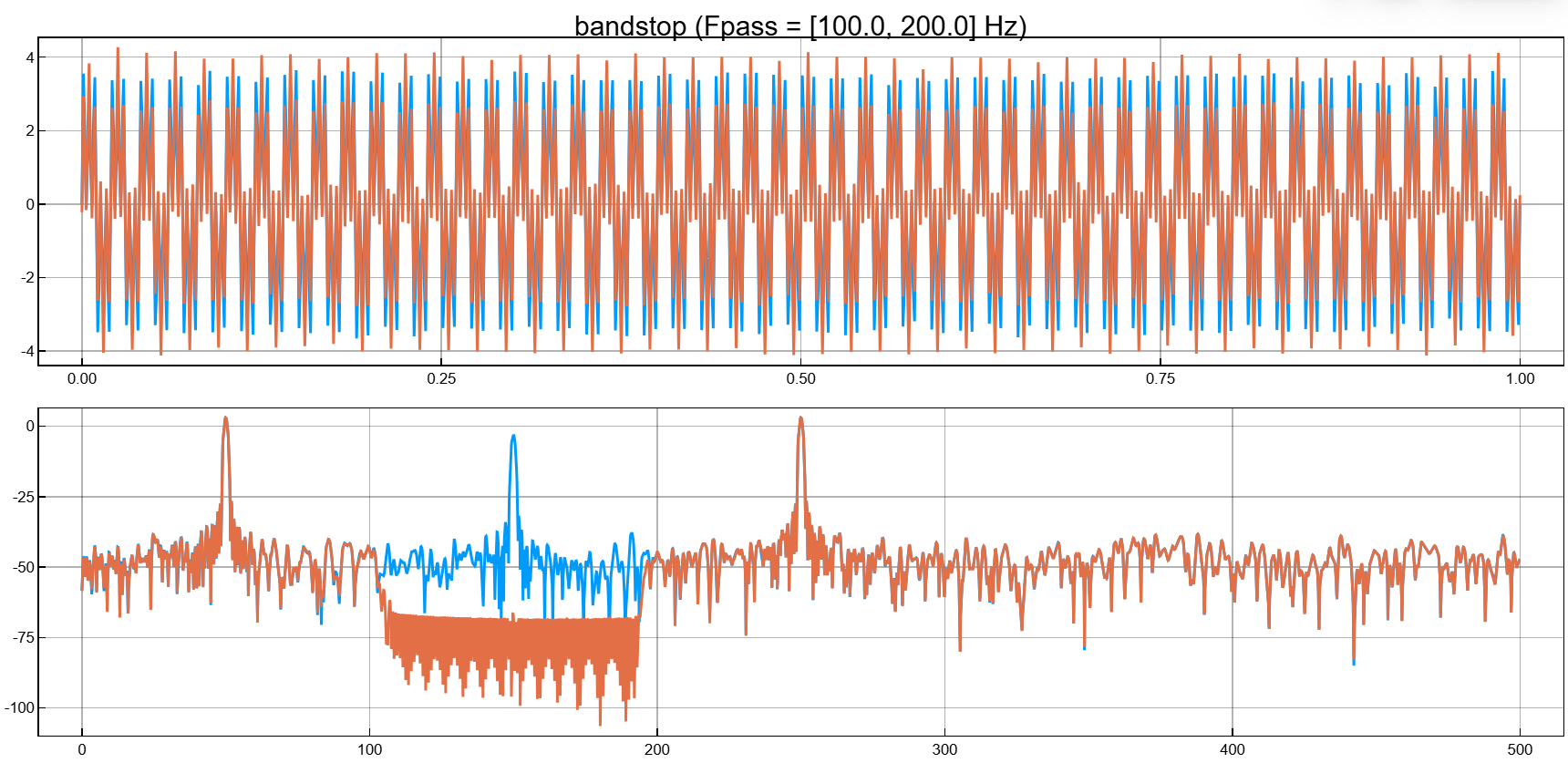
The steepness of the decline of the notch filter
Details
Filter out the white noise sampled with the frequency 1 kHz, using a notch filter with infinite pulse response and delay band 100 Hz. We use different values of steepness. Let’s plot the spectra of the filtered signals.
import EngeeDSP.Functions: randn, bandstop, pspectrum

fs = 1000;
x = randn(20000,1);

y1 = bandstop(x,[50 150],fs,"ImpulseResponse","iir","Steepness",0.5)
y2 = bandstop(x,[200 300],fs,"ImpulseResponse","iir","Steepness",0.8)
y3 = bandstop(x,[350 450],fs,"ImpulseResponse","iir","Steepness",0.95)

pspectrum([y1 y2 y3],fs,out=:plot)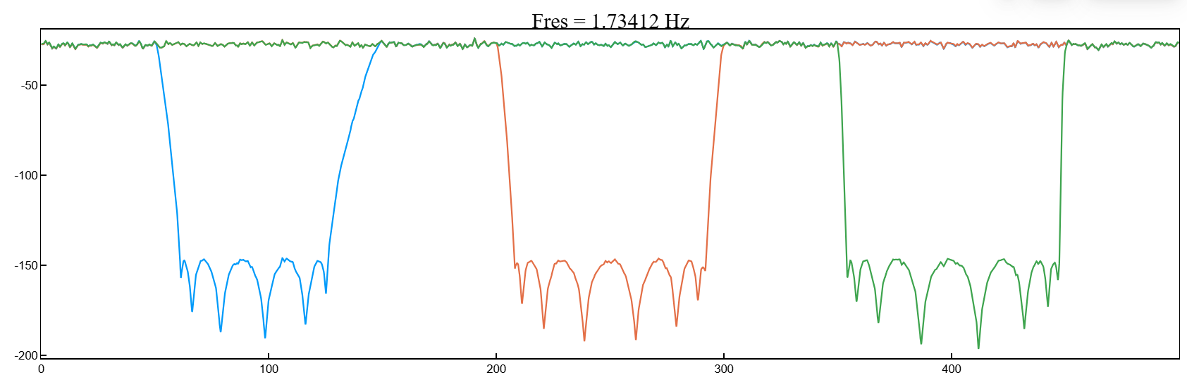
Let’s make the filters asymmetric by setting different steepness values at the lower and upper frequencies of the delay band.
y1 = bandstop(x,[50 150],fs,"ImpulseResponse","iir","Steepness",[0.5 0.8])
y2 = bandstop(x,[200 300],fs,"ImpulseResponse","iir","Steepness",[0.5 0.8])
y3 = bandstop(x,[350 450],fs,"ImpulseResponse","iir","Steepness",[0.5 0.8])

pspectrum([y1 y2 y3],fs,out=:plot)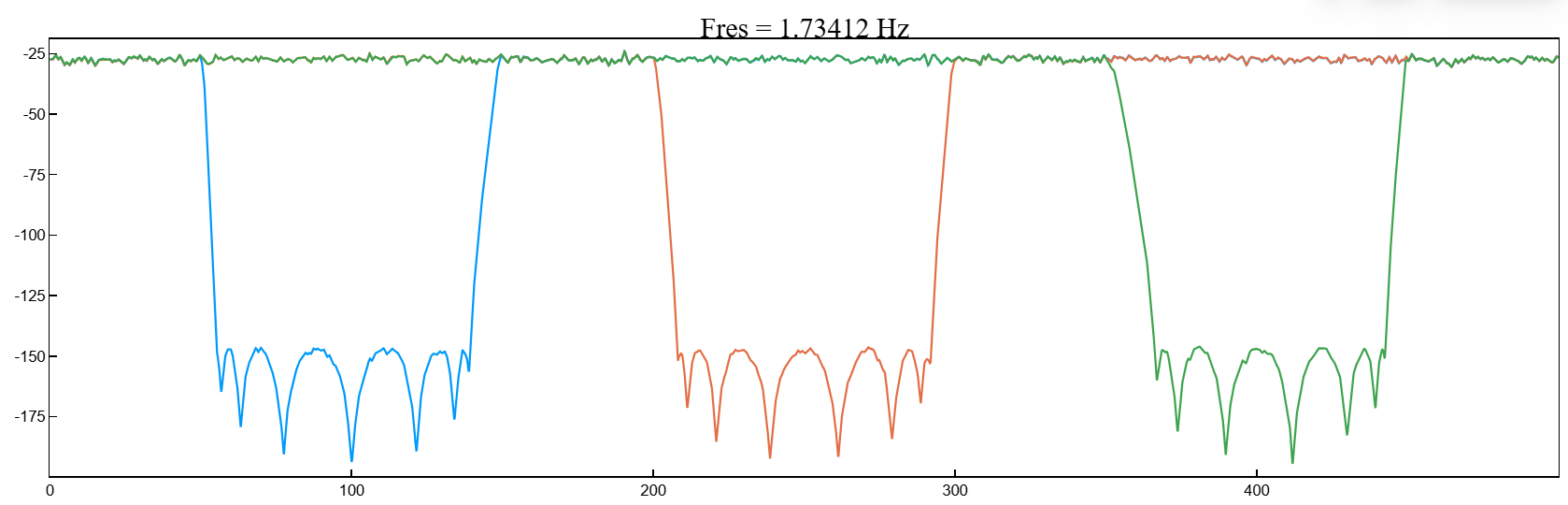
Additional Info
The steepness of the decline of the notch filter
Details
Argument Steepness controls the width of the filter transition areas. The lower the slope, the wider the transition area. The higher the steepness, the narrower the transition area will be.
To interpret the steepness of the filter, consider the following definitions:
-
_ Nyquist Frequency_ — the highest frequency component of the signal that can be sampled at a given frequency without distortion. The Nyquist frequency is rad/countdown if the input signal does not contain time information, and Hz, if you set the sampling rate.
-
The lower and upper frequencies of the delay band_ of the filter and — frequencies below and above which the attenuation is equal to or greater than the value set using
StopbandAttenuation.The center of the holding lane .
-
_ Width of the lower transition band_ of the filter , where — the first element of the set frequencies
fpass. -
_ Width of the upper transition band_ of the filter , where — the second element of the set frequencies
fpass. -
Most imperfect filters also attenuate the input signal in the bandwidth. The maximum value of this frequency-dependent attenuation is called the bandwidth pulsation. Each filter used in the function
bandstopit has ripples in the bandwidth0.1dB.

To control the width of the transition strips, you can specify an argument Steepness as a two-element vector , or as a scalar.
When Steepness set as a vector:
-
The function calculates the width of the lower transition band as
-
The function calculates the width of the upper transition band as
When is the argument Steepness given as a scalar, then the function:
-
Calculates and using the specified scalar value.
-
Creates a symmetrical filter with the width of the lower and upper transition bands equal to the smaller of the and .
The default value of the argument is Steepness equally [0.85 0.85].