residuez
Decomposition of the Z-transform into simple fractions.
| Library |
|
Arguments
Input arguments
# bi,ai — coefficients of the polynomial
+
vectors
Details
Coefficients of the polynomial, set as vectors. Vectors b and a coefficients of polynomials of discrete systems are set in ascending order of degrees :
If there are several roots and Then
# ri — deductions of decomposition into simple fractions
+
column vector
Details
The deductions of the decomposition into simple fractions, given as a vector.
# pi — poles of decomposition into simple fractions
+
column vector
Details
Poles of decomposition into simple fractions, given as a vector.
# ki — the polynomial of the integer part of the decomposition
+
vector string
Details
The polynomial of the integer part of the expansion, defined as a vector.
Output arguments
# ro — deductions of decomposition into simple fractions
+
column vector
Details
The deductions of the decomposition into simple fractions returned as a vector.
# po — poles of decomposition into simple fractions
+
column vector
Details
The poles of the decomposition into simple fractions returned as a vector.
The number of poles is defined as
If is the pole of multiplicity , that decomposition includes terms of the form
# ko — the polynomial of the integer part of the decomposition
+
vector string
Details
The polynomial of the integer part of the expansion, returned as a vector.
Vector of coefficients of the polynomial of the whole part empty if less ; otherwise:
# bo,ao — coefficients of the polynomial
+
vectors
Details
Coefficients of the polynomial returned as vectors.
Examples
Decomposition into simple fractions of the IIR low-pass filter
Details
Let’s calculate the decomposition into simple fractions corresponding to the third-order IIR low-pass filter described by the transfer function
Let’s express the numerator and denominator in the form of polynomial convolutions.
import EngeeDSP.Functions: conv, residuez

b0 = 0.05634
b1 = [1, 1]
b2 = [1, -1.0166, 1]
a1 = [1, -0.683]
a2 = [1, -1.4461, 0.7957]

b = b0*conv(b1,b2)
a = conv(a1,a2)
Let’s calculate the deductions, poles, and the polynomial of the integer part of the decomposition into simple fractions.
r,p,k = residuez(b,a)

print("r: ")
show(stdout, "text/plain", r)
println()
print("p: ")
show(stdout, "text/plain", p)
println()
print("k: ")
show(stdout, "text/plain", k)
r: 3×1 Matrix{ComplexF64}:
-0.1152524739870425 - 0.018151109860882933im
-0.1152524739870425 + 0.018151109860882933im
0.39051343991033616 + 0.0im
p: 3×1 Matrix{ComplexF64}:
0.7230499999999996 + 0.522397068808775im
0.7230499999999996 - 0.522397068808775im
0.6829999999999996 - 0.0im
k: -0.10366849193625106Let’s plot the poles and zeros of the transfer function and superimpose the poles found on it.
zeros = roots(vec(b))
poles = roots(vec(a))
θ = range(0, 2π, length=100)
unit_circle = exp.(1im * θ)

plot(real(unit_circle), imag(unit_circle),
     linecolor=:black,
     linestyle=:dash,
     label="Unit Circle",
     aspect_ratio=:equal,
     xlims=(-1.2, 1.2),
     ylims=(-1.2, 1.2))

scatter!(real(zeros), imag(zeros),
         marker=:circle,
         markersize=8,
         color=:blue,
         label="b")

scatter!(real(poles), imag(poles),
         marker=:circle,
         markersize=8,
         color=:red,
         label="a")

scatter!(real(p), imag(p),
         marker=:x,
         markersize=5,
         color=:green,
         label="poles")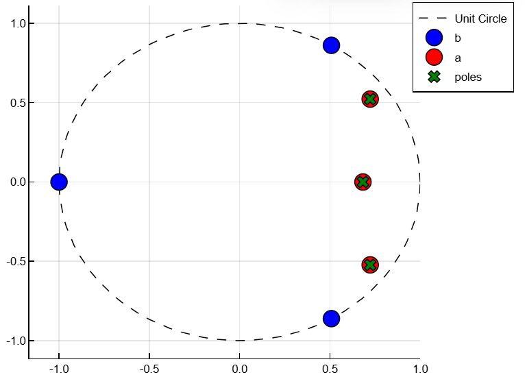
We use residuez again, to restore the transfer function.
bn,an = residuez(r,p,k)
print("bn: ")
show(stdout, "text/plain", bn)
println()
print("an: ")
show(stdout, "text/plain", an)
bn: 1×4 Matrix{Float64}:
0.05634 -0.000935244 -0.000935244 0.05634
an: 1×4 Matrix{Float64}:
1.0 -2.1291 1.78339 -0.543463Algorithms
Function residuez converts a discrete system expressed as a ratio of two polynomials into a prime fraction decomposition. It also converts the decomposition into simple fractions back to the original coefficients of the polynomial.
| From a numerical point of view, decomposing the ratio of polynomials into simple fractions is an incorrect task. If the polynomial in the denominator is close to a polynomial with multiple roots, then small changes in the data, including rounding errors, can lead to arbitrarily large changes in the resulting poles and subtractions. Instead, state space representations or representations with poles and zeros should be used. |
Function residuez applies standard functions Engee and methods of the simplest fractions for finding r, p and k from b and a. She finds:
-
The polynomial of the integer part of the decomposition
awith the helpdeconv(polynomial division) whenlength(b) > length(a) − 1. -
Poles using
p = roots(a). -
Any multiple poles, rearranging the poles according to their multiplicity.
-
Deduction for each simple pole by multiplication on and calculating the resulting rational function for .
-
Deductions for multiples of poles by solving
for using an operation
\. Here — the impulse response of the reduced , — a matrix, the columns of which represent the impulse characteristics of first-order systems consisting of simple roots, and — a column containing deductions for simple roots. Each column of the matrix It represents an impulse response. For each root multiplicities the matrix contains columns representing the impulse characteristics of each of the following systems:Vector and matrices and they have lines where — the total number of roots, and the internal parameter , by default equal to
1, determines the degree of redefinition of the system of equations.