ss2sos
Transformation of digital filter parameters in the state space into second-order sections.
| Library |
|
Arguments
Input arguments
# A is the state matrix
+
the matrix
Details
The state matrix, defined as a matrix. If the system has entrances and outputs and is described by state variables, then the matrix A has a size of on .
# B is the entry matrix
+
the matrix
Details
The input matrix, set as a matrix. If the system has entrances and outputs and is described by state variables, then the matrix B has a size of on .
# C is the output matrix
+
the matrix
Details
The output matrix, set as a matrix. If the system has entrances and outputs and is described by state variables, then the matrix C has a size of on .
# D is the end—to- end transmission matrix
+
the matrix
Details
The end-to-end transmission matrix, defined as a matrix. If the system has entrances and outputs and is described by state variables, then the matrix D has a size of on .
# scale — scaling of the gain and numerator
+
"none" (by default) | "inf" | "two"
Details
Scaling of the gain coefficients and numerator, set to one of the following values:
-
"none"— scaling is not applied; -
"inf"— infinite rate scaling; -
"two"— scaling according to the second norm.
Using infinite norm scaling with order "up" minimizes the chance of overflow in the implementation. Using scaling according to the second norm with an order "down" minimizes peak rounding noise.
| Scaling by the infinite norm and by the second norm is suitable only for implementations in direct form II. |
Output arguments
# sos — representation of the second-order section
+
the matrix
Details
The representation of the second-order section, returned as a matrix. Argument sos — this is a matrix of size
the rows of which contain the coefficients of the numerator and denominator and second-order sections of the function :
# g is the total gain of the system
+
scalar
Details
The total gain of the system, returned as a real scalar.
If you call the function ss2sos With one output argument, the function will embed the total gain of the system into the first section. So that
Embedding the gain in the first section when scaling a straight-form II structure is not recommended and may lead to unstable scaling. To avoid embedding the gain factor, use ss2sos with two output arguments: sos and g.
|
Examples
Representation of the filter in the form of second-order sections
Details
Let’s develop a 5th-order Butterworth low-pass filter by setting the cutoff frequency to rad/count and representing the output signal in the form of a state space. We transform the result in the state space into second-order sections. Visualize the frequency response of the filter.
import EngeeDSP.Functions: butter, ss2sos

A, B, C, D = butter(5, 0.2, out = 4)
sos, g = ss2sos(A, B, C, D)
println("sos = ", sos)
sos = [1.0 1.0004631991200947 0.0 1.0 -0.5095254494944288 0.0; 1.0 1.9995370439927413 0.9995370439927413 1.0 -1.0965794655679613 0.35544676217239035; 1.0 1.999999756887197 0.9999999713279842 1.0 -1.3693171946832927 0.6925691353878634]import EngeeDSP.Functions: freqz
freqz(sos, out = :plot)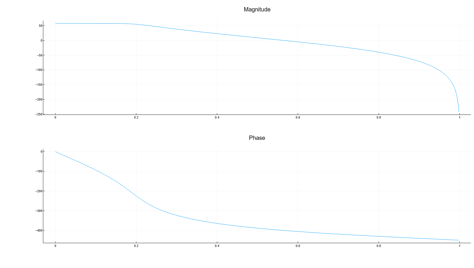
Mass-spring system
Details
A one-dimensional discrete oscillatory system consists of a single mass , attached to the wall by a spring with a unit elastic constant . The sensor registers acceleration masses with frequency Hz.

Generate 50 sampling periods. Let’s define the sampling interval .
Fs = 5
dt = 1 / Fs
N = 50
t = dt * (0:N-1)
The oscillator can be described by the equations of the state space:
where — the state vector, and — respectively, the position and velocity of the mass, and the matrix
A = [cos(dt) sin(dt); -sin(dt) cos(dt)]
B = [1 - cos(dt); sin(dt)]
C = [-1 0]
D = 1
The system is excited by a single pulse in the positive direction. We use the state space model to calculate the time evolution of the system, starting from the zero initial state.
u = [1; zeros(N-1)]

x = [0.0; 0.0]
y = zeros(N)

for k = 1:N
    y[k] = (C * x)[1] + D * u[k]
    global x = A * x + B * u[k]
end
Let’s plot the dependence of mass acceleration on time.
plot(t, y,
     seriestype = :stem,
     marker = :circle,
     legend = false)
Let’s calculate the dependence of acceleration on time using the transfer function to filter the input signal. Let’s express the transfer function in the form of second-order sections. Let’s plot the result graph. The result is the same in both cases.
import EngeeDSP.Functions: ss2sos, sosfilt

sos = ss2sos(A, B, C, D)
yt = sosfilt(sos[1], u)
plot(t, yt,
     seriestype = :stem,
     marker = :circle,
     legend = false)
Algorithms
Function ss2sos uses a four-step algorithm to determine the representation of a second-order section for the input state space system:
-
It finds the poles and zeros of the system specified by the parameters
A,B,CandD. -
Uses the function
zp2sos, which first groups the zeros and poles into complex conjugate pairs using the functioncplxpair. Thenzp2sosforms second-order sections by combining pairs of poles and zeros in accordance with the following rules:-
Combine the poles closest to the unit circle with the zeros closest to these poles.
-
Combine the poles closest to the unit circle with the zeros closest to these poles.
-
Continue until all poles and zeros are combined.
Function
ss2sosgroups the real poles into sections where the real poles are closest to them in absolute value. The same rule applies for real zeros. -
-
Arranges the sections according to the proximity of the pairs of poles to the unit circle. Usually
ss2sosarranges the sections with poles closest to the unit circle, the last in the cascade. You can specify functionsss2sosso that it orders the sections in reverse order using the argumentorder. -
Function
ss2sosscales sections according to the norm specified in the argumentscale. For an arbitrary function The scaling is defined as follows:where it can be either infinite, or
2. For more information about scaling, see in the sources in the Literature section. The algorithm follows this scaling to minimize overflow or peak rounding noise in fixed-point filter implementations.
Literature
-
Jackson, L. B. Digital Filters and Signal Processing. 3rd ed. Boston: Kluwer Academic Publishers, 1996.
-
Mitra, S. K. Digital Signal Processing: A Computer-Based Approach. 3rd ed. New York: McGraw-Hill Higher Education, 2006.
-
Vaidyanathan, P. P. «Robust Digital Filter Structures.» Handbook for Digital Signal Processing (S. K. Mitra and J. F. Kaiser, eds.). New York: John Wiley & Sons, 1993.