fillgaps
Filling gaps using autoregression modeling.
| Library |
|
Syntax
Arguments
Input arguments
# x — input signal
+
vector | the matrix
Details
An input signal specified as a vector or matrix. If x is a matrix, then its columns are treated as independent channels. The signal x contains values NaN to represent the missed counts.
| Data types |
|
| Support for complex numbers |
Yes |
# maxlen — maximum length of prediction sequences
+
a positive integer
Details
The maximum length of the prediction sequences, set as a positive integer. If you don’t ask maxlen Then fillgaps iteratively selects autoregression models, using all previous points for direct estimation and all future points for reverse estimation.
| Data types |
|
# order — the order of the autoregression model
+
a positive integer
Details
The order of the autoregression model, set as a positive integer. The order is truncated if order infinite or if there are not enough available counts. If you don’t ask order Then fillgaps selects the order that minimizes the Akaike information criterion.
| Data types |
|
Output arguments
# y — reconstructed signal
+
vector | the matrix
Details
The reconstructed signal returned as a vector or matrix.
Examples
Filling gaps in functions
Details
Let’s generate a function consisting of the sum of two sinusoids and a Lorentz curve. The function is sampled with frequency 200 Hz during 2 seconds. Let’s build a graph.
import EngeeDSP.Functions: fillgaps

x = -1:0.005:1
f = 1 ./ (1 .+ 10 .* x.^2) .+ sin.(2*pi*3*x)/10 .+ cos.(25*pi*x)/10

plot(x, f)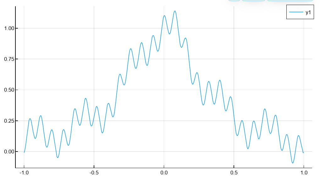
Let’s insert gaps in the intervals (−0.8,−0.6), (−0.2,0.1) and (0.4,0.7).
h = copy(f)

h[(x .> -0.8) .& (x .< -0.6)] .= NaN
h[(x .> -0.2) .& (x .< 0.1)] .= NaN
h[(x .> 0.4) .& (x .< 0.7)] .= NaN
Fill in the gaps using the default settings fillgaps. Let’s plot the original and reconstructed functions.
y = fillgaps(h)

plot(x, f, seriestype = :scatter, markersize = 2, color = :blue, label = "Original")
plot!(x, y, linewidth = 2, color = :red, label = "Reconstructed")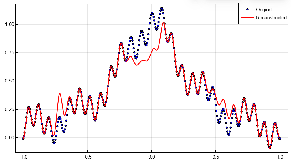
Let’s repeat the calculations, but now we’ll set the maximum length of the prediction sequence. 3 reference points and the order of the model 1. Let’s plot the graphs of the original and reconstructed functions. In the simplest case fillgaps performs a linear approximation.
y = fillgaps(h,3,1)

plot(x, f, seriestype = :scatter, markersize = 2, color = :blue, label = "Original")
plot!(x, y, linewidth = 2, color = :red, label = "Reconstructed")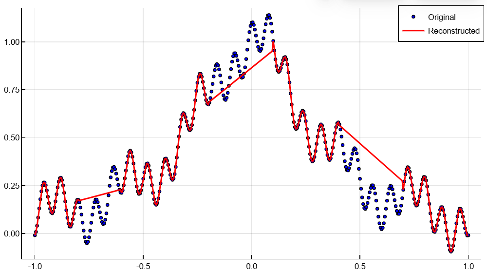
Setting the maximum length of the prediction sequence 80 counts and the order of the model 40. Let’s plot the graphs of the original and reconstructed functions.
y = fillgaps(h,80,40)

plot(x, f, seriestype = :scatter, markersize = 2, color = :blue, label = "Original")
plot!(x, y, linewidth = 2, color = :red, label = "Reconstructed")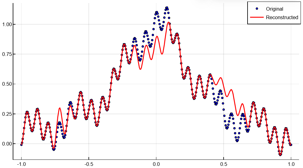
Let’s change the order of the model to 70. Let’s plot the graphs of the original and reconstructed functions.
y = fillgaps(h,80,70)

plot(x, f, seriestype = :scatter, markersize = 2, color = :blue, label = "Original")
plot!(x, y, linewidth = 2, color = :red, label = "Reconstructed")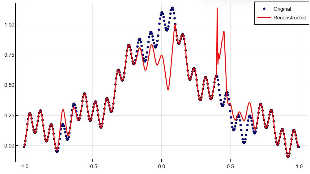
The reconstruction is imperfect, because at very high model orders there are often problems with finite accuracy.
Literature
-
Akaike, Hirotugu. Fitting Autoregressive Models for Prediction. Annals of the Institute of Statistical Mathematics. Vol. 21, 1969, pp. 243–247.
-
Kay, Steven M. Modern Spectral Estimation: Theory and Application. Englewood Cliffs, NJ: Prentice Hall, 1988.
-
Orfanidis, Sophocles J. Optimum Signal Processing: An Introduction. 2nd Edition. New York: McGraw-Hill, 1996.