freqz

Frequency response of a digital filter.

Library

EngeeDSP

Syntax

Function call

h,w = freqz(b,a,n) — returns the frequency response of the specified digital filter. Specify a digital filter with numerator coefficients b and the coefficients of the denominator a. The function returns n-the point vector of the frequency response in the output argument h and the corresponding vector of angular frequencies w.

h,w = freqz(B,A,ctf=true,n) — returns n-the point frequency response of the digital filter, represented as Cascaded Transfer Functions (CTF) with numerator coefficients B and the coefficients of the denominator A.

h,w = freqz((B,A,g),ctf=true,n) — returns n-the dot frequency response of the digital filter in CTF format. Specify a filter with numerator coefficients B, the coefficients of the denominator A and scale values g by filter sections.

h,w = freqz(sos,n) — returns n-a point-based complex frequency response corresponding to a matrix of second-order sections sos.

h,w = freqz(___,n,"whole") — returns n-the point frequency response of the sample over the entire unit circle.

h,f = freqz(___,n,fs) — returns the frequency response vector h and the corresponding vector of physical frequencies f for a digital filter designed to filter signals sampled with frequency fs.

h,f = freqz(___,n,"whole",fs) — returns the frequency vector in n points in the range from 0 before fs.

h = freqz(___,w) — returns the frequency response vector h calculated on the normalized frequencies specified in the input argument w.

h = freqz(___,f,fs) — returns the frequency response vector h calculated at the physical frequencies specified in the input argument f.

freqz(___,out=:plot) — plots the frequency response of the filter.

Arguments

Input arguments

# b,a are the coefficients of the transfer function

+ vectors

Details

The coefficients of the transfer function, set as vectors. The transfer function is expressed in terms of b and a as follows:

Типы данных	`Float64`, `Float32`
Support for complex numbers	Yes

# n is the number of frequency points by which the characteristic is evaluated

+ 512 (by default) | a positive integer

Details

The number of frequency points by which the characteristic is evaluated, set as a positive integer of at least 2. If the argument is n not specified, the default value is 512. For best results, set for the argument n a value exceeding the filter order.

# B,A are the coefficients of the cascade transfer function

+ scalars | vectors | matrices

Details

The coefficients of the cascade transfer function, specified as scalars, vectors, or matrices. In matrices B and A The coefficients of the numerator and denominator of the cascade transfer function are listed, respectively.

The matrix B must have a size of on , and the matrix A — on , where

— number of filter sections;
— the order of the numerators of the filter;
— the order of the denominators of the filter.

For more information about the cascade transfer function format and coefficient matrices, see Setting digital filters in CTF format.

If any element of the matrix A[:,1] not equal to 1, then the function freqz normalizes the filter coefficients by A[:,1]. In this case A[:,1] it must be non-zero.

Типы данных	`Float64`, `Float32`
Support for complex numbers	Yes

# g — scale values

+ scalar | vector

Details

Scale values specified as a real scalar or vector with real values containing the element where — the number of sections of the cascade transfer function. The scale values represent the distribution of the filter gain across the sections of the cascade filter representation.

Function freqz applies the gain to the filter sections using the function scaleFilterSections depending on the way the argument is set g:

scalar — the function evenly distributes the gain across all sections of the filter;
vector — the function applies the first applies the gain values to the corresponding filter sections and distributes the last gain value evenly across all filter sections.

Типы данных

Float64, Float32

# sos — coefficients of the sections of the second order

+ the matrix

Details

Coefficients of the second-order sections, specified as a matrix. Argument sos — this is a matrix of size on , where is the number of sections must be greater than or equal to 2. If the number of sections is less 2, the function processes the input data as a vector of numerators. Each line sos corresponds to the coefficients of the second-order filter (biquadrate filter); - I’m a string sos respond [bi[1] bi[2] bi[3] ai[1] ai[2] ai[3]].

Типы данных	`Float64`, `Float32`
Support for complex numbers	Yes

# fs — sampling rate
scalar

Details

The sampling rate, set as a positive scalar. If the unit of time is seconds, then fs expressed in Hz.

Типы данных

Float64

# w — angular frequencies

+ vector

Details

The angular frequencies are set as a vector, and the units of measurement are rad/count. Vector w it must contain at least two elements, otherwise the function interprets it as n. The value of the argument w = π corresponds to the Nyquist frequency.

# f — frequencies

+ vector

Details

Frequencies specified as a vector. Vector f it must contain at least two elements, otherwise the function interprets it as n. If the unit of time is seconds, then f expressed in Hz.

Типы данных

Float64

Name-value input arguments

Specify optional argument pairs as Name=Value, where Name — the name of the argument, and Value — the appropriate value.

# ctf — cascade transfer function

+ false (default) | true

Details

Frequency response output format:

false — the function returns the frequency response of the digital filter;
true — the function returns the frequency response of the digital filter, represented as cascaded transfer functions.

For more information, see Cascading transfer functions.

Типы данных

Bool

# out — type of output data

+ :data (default) | :plot

Details

Type of output data:

:data — the function returns data;
:plot — the function returns a graph.

Output arguments

# h — frequency response

+ vector

Details

The frequency response returned as a vector. If the argument is n if set, then the vector h has a length of n. If n if it is not specified or set as an empty vector, then the length of the vector is h equal to 512.

If the input data of the function is freqz they have single precision, the function calculates the frequency response using single precision arithmetic. Output argument h it has a single precision.

# w — angular frequencies

+ vector

Details

The angular frequencies returned as a vector. The value of the argument w varies from 0 before . If an argument is given as input "whole", then the values in the vector w will vary from 0 before . If an argument is given n, vector w has a length of n. If n if it is not specified or set as an empty vector, then the length of the vector is w equal to 512.

# f — frequencies

+ vector

Details

Frequencies returned as a vector and expressed in Hz. Argument f accepts values from 0 before fs/2 Hz. If an argument is given as input "whole", then the values in the vector f will be in the range of 0 before fs Hz. If an argument is given n, vector f has a length of n. If n if it is not specified or set as an empty vector, then the length of the vector is f equal to 512.

Examples

Frequency response of the transfer function

Details

Let’s calculate and display the amplitude-frequency response of the IIR low-pass filter of the third order, described by the following transfer function:

Let’s express the numerator and denominator in the form of polynomial convolutions. Let’s find the frequency response in 2001 a point that covers the entire unit circle.

import EngeeDSP.Functions: conv, freqz

b0 = 0.05634
b1 = [1  1]
b2 = [1 -1.0166 1]
a1 = [1 -0.683]
a2 = [1 -1.4461 0.7957]

b = b0 * conv(b1, b2)
a = conv(a1, a2)

h, w = freqz(b, a, "whole", 2001)

Let’s plot the amplitude-frequency response, expressed in dB.

plot(w./(maximum(w)/2), 20*log10.(abs.(h)),
     xlabel = "Normalized Frequency (×π rad/sample)",
     ylabel = "Magnitude (dB)",
     legend = false,
     ylims = (-100, 20))

freqz 1

Frequency response of the FIR filter

Details

Let’s design a low-pass FIR filter 80-th order, using the Kaiser window with . Setting the normalized cutoff frequency rad/countdown. Let’s display the amplitude-frequency and phase characteristics of the filter.

import EngeeDSP.Functions: fir1, kaiser, freqz

b = fir1(80, 0.5, kaiser(81, 8))

freqz(b, 1, out = :plot)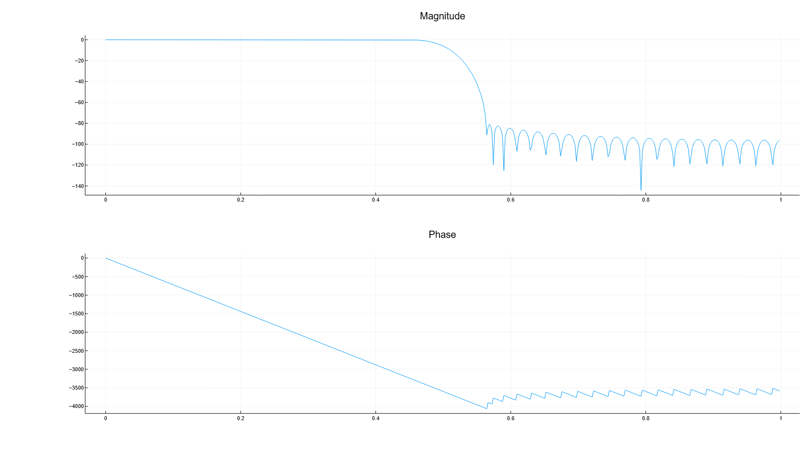

freqz 2

Frequency response of second-order sections

Details

Let’s calculate and display the amplitude-frequency response of the IIR low-pass filter of the third order, described by the following transfer function:

Let’s express the transfer function in terms of second-order sections. Let’s find the frequency response in 2001 a point that covers the entire unit circle.

import EngeeDSP.Functions: freqz

b0 = 0.05634
b1 = [1  1]
b2 = [1 -1.0166 1]
a1 = [1 -0.683]
a2 = [1 -1.4461 0.7957]

sos1 = [b0*[b1 0] [a1 0]]
sos2 = [b2 a2]

h, w = freqz([sos1; sos2], "whole", 2001)

Let’s plot the amplitude-frequency response, expressed in dB.

plot(w./(maximum(w)/2), 20*log10.(abs.(h)),
     xlabel = "Normalized Frequency (×π rad/sample)",
     ylabel = "Magnitude (dB)",
     legend = false,
     ylims = (-100, 20))

freqz 3

Additional Info

Cascading transfer functions

Details

Splitting a digital IIR filter into cascaded sections increases its numerical stability and reduces its susceptibility to coefficient quantization errors. Cascade form of the transfer function in terms of transfer functions it has the form

butter en

Setting digital filters in CTF format

Details

Digital filters can be designed in CTF format to analyze, visualize, and filter signals. The filter is set by enumerating its coefficients B and A. You can also specify the scaling factor of the filter by sections by setting a scalar or vector value. g.

coeffects of the filter

When setting coefficients in the form -lowercase matrices

it is assumed that the filter is set as a sequence of cascade transfer functions, so that the complete transfer function of the filter has the form

where — the order of the filter numerator, and — the order of the denominator.

If and defined as vectors, it is assumed that the basic system is a single-section IIR filter ( ), where represents the numerator of the transfer function, and — its denominator.
If — scalar, it is assumed that the filter is a cascade of IIR filters with poles, and the total gain of the system of each cascade is equal to .
If — scalar, it is assumed that the filter is a cascade of FIR filters, and the total gain of the system of each cascade is equal to .

To convert second-order section matrices into cascade transfer functions, use the function sos2ctf.
To convert the filter representation with zeros, poles, and gain into cascaded transfer functions, use the function zp2ctf.

coeffects and amplification

If there is a common scale gain or several scale gain factors that are outside the values of the filter coefficients, you can specify the coefficients and gain as a tuple. (B, A, g). Scaling the filter sections is especially important when working with fixed-point arithmetic to ensure that the output signals of each filter section have similar amplitude levels, which helps to avoid inaccuracies in the frequency response of the filter due to limited computational accuracy.

The gain can be a scalar total gain or a vector of section gain coefficients.

If the gain is scalar, its value is applied uniformly to all sections of the cascade filter.
If the gain is a vector, it must contain one element more than the number of filter sections. in the cascade. Each of the first The scale value is applied to the corresponding filter section, and the last value is applied evenly to all sections of the cascade filter.

If you specify the filter coefficient matrices and the gain coefficient vector as

it is assumed that the transfer function of the filter system has the form

Algorithms

The frequency response of a digital filter can be interpreted as a transfer function calculated at a point [1].

Function freqz defines the transfer function from the numerator and denominator polynomials you specified (real or complex) and returns the complex frequency response a digital filter. The frequency response is calculated at the sampling points determined by the syntax you use.

Function freqz It usually uses the FFT algorithm to calculate the frequency response if no frequency vector is specified as the input argument. It calculates the frequency response as the ratio of the converted coefficients of the numerator and denominator, padded with zeros to the desired length.

If the frequency vector is specified as the input argument, the function freqz calculates the values of the polynomials at each frequency point and divides the value of the characteristic of the numerator by the value of the characteristic of the denominator. To calculate the values of the polynomials, the function uses the Horner method.

Literature

Oppenheim, Alan V., and Ronald W. Schafer, with John R. Buck. Discrete-Time Signal Processing. 2nd Ed. Upper Saddle River, NJ: Prentice Hall, 1999.
Lyons, Richard G. Understanding Digital Signal Processing. Upper Saddle River, NJ: Prentice Hall, 2004.