sgolay
Calculation of the Savitsky—Goley filter.
| Library |
|
Arguments
Output arguments
# b — FIR filter coefficients that change over time
+
the matrix
Details
FIR filter coefficients, time-varying, returned as a matrix fl×fl. In the implementation of the smoothing filter, the last (fl−1)/2 rows (each with a filter) are applied to the signal during the initial transient, and the first (fl−1)/2 rows — during the final transition process. The center line is applied to the steady state signal.
# g is a matrix of differential filters
+
the matrix
Details
The matrix of differential filters. Each column g It is a differential filter for derivatives of order p−1, where p — index of the column. If a signal is set x lengths fl you can find an estimate of the derivative p- th order, xp, its average value from xp((fl+1)/2) = factorial(p) * (g[:, p+1]' * x).
Examples
Smoothing of a noisy sinusoid using the Savitsky—Goley method
Details
We will generate a signal representing a sinusoid with a frequency of 0.2 Hz, to which white Gaussian noise is added, at a sampling rate of five times per second during 200 seconds.
import EngeeDSP.Functions: randn, sgolay,conv

dt = 1/5
t = (0:dt:200-dt)'
x = 5*sin.(2*pi*0.2*t) + randn(1, length(t))
We use sgolay to smooth the signal. We use frames from 21 counting and polynomials of the fourth degree.
order = 4
framelen = 21
b,g = sgolay(order,framelen)
Calculate the steady-state part of the signal by convolving it with the middle row of the vector b.
ycenter = conv(x,b[Int((framelen+1)/2), :],"valid")'Let’s calculate the transients. We use the last rows of the matrix b to start and the first rows of the matrix b for completion.
ybegin = b[end:-1:Int((framelen+3)/2), :] * x[framelen:-1:1]
yend = b[Int((framelen-1)/2):-1:1, :] * x[end:-1:end-(framelen-1)]
Let’s combine the transients and the steady-state part of the signal to get a complete smoothed signal. Let’s plot the original signal and the signal smoothed using the Savitsky—Goley method.
y = [ybegin; ycenter; yend]

plot(x', label = "Noisy Sinusoid")
plot!(y, label = "S-G smoothed sinusoid")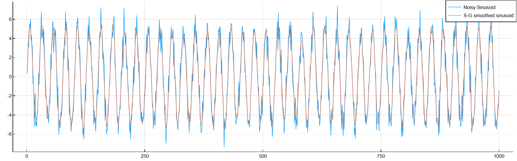
Savitsky — Goley filter with scales
Details
Let’s design a Savitsky—Goley smoothing filter with polynomials 5`to filter a noisy signal sampled with a frequency of `8192 Hz. We use the Hamming window. The frame length is 101 the countdown.
import EngeeDSP.Functions: hamming, freqz, sgolay

Fs = 8192
m = 5
fl = 101
weights = hamming(fl)
b,g = sgolay(m,fl,weights)
Let’s construct the frequency response for the central line b. We use 1024 FFT points.
NFFT = 1024
b=b[Int((fl+1)/2), :]
freqz(b',1,NFFT,Fs,out=:plot)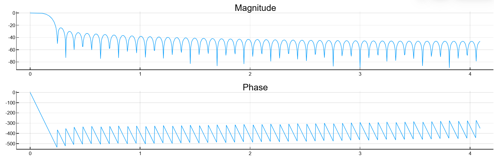
Savitsky—Goley differentiation
Details
We will generate a signal representing a sinusoid with a frequency of 0.2 Hz, to which white Gaussian noise is added, at a sampling rate of four times per second during 20 seconds.
import EngeeDSP.Functions: randn, sgolay,conv

dt = 0.25
t = (0:dt:20-1)'
x = 5*sin.(2*pi*0.2*t) + 0.5*randn(1, length(t))
Let’s evaluate the first three derivatives of the sine wave using the Savitsky—Goley method. We use 25-point windows and fifth-order polynomials. Let’s divide the columns into degrees dt to scale the derivatives correctly.
b,g = sgolay(5,25)

dx = zeros(length(x), 4)
for p in 0:3
    kernel = factorial(p) / (-dt)^p * g[:, p+1]
    dx[:, p+1] = conv(x, kernel, "same")
end
Let’s plot the original signal, the smoothed sequence, and the derivatives.
plot(x', marker = :., label = "x")
plot!(dx, label = ["x (smoothed)" "x'" "x''" "x'''"])
title!("Savitzky-Golay Derivative Estimates")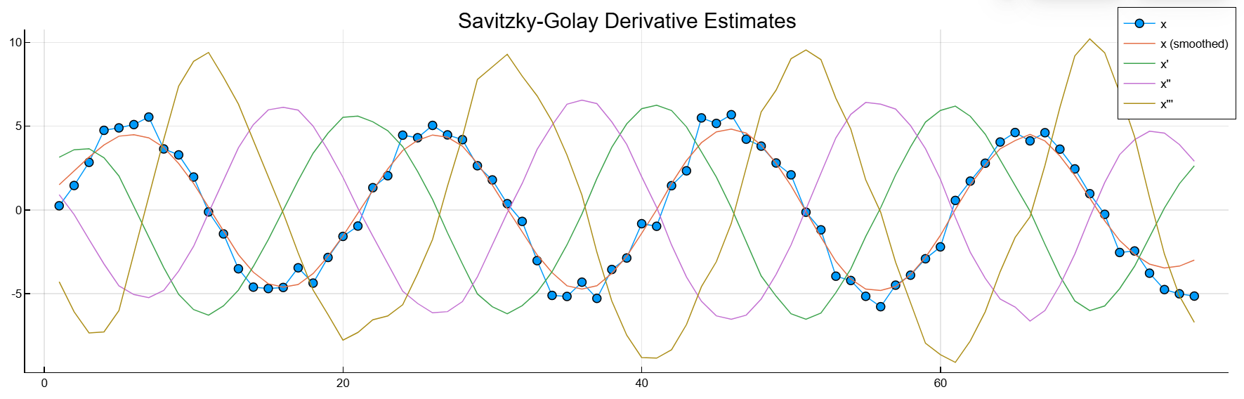
Algorithms
Savitsky—Goley filters are used to smooth out noisy signals with a large frequency range. Savitsky—Goley smoothing filters, as a rule, filter out less of the high-frequency content of the signal than standard FIR averaging filters. However, they are less effective at suppressing noise when its level is particularly high.
In general, filtering consists of replacing each signal point with some combination of signal values contained in a sliding window centered at that point, based on the assumption that nearby points measure almost the same base value. For example, moving average filters replace each data point with a local average of the surrounding data points. If the data point has points on the left and points on the right, for the total length of the window , then the moving average filter makes a replacement
Savitsky—Goley filters generalize this idea by approximating order polynomials using the least squares method. to the values of the signal in the window and taking the calculated center point of the polynomial curve as a new smoothed data point. For a given point
or, in terms of matrices,
To find the Savitsky—Goley estimates, we use the pseudoinversion to calculate , and then multiply from the left by :
To avoid bad conditioning, the function sgolay uses QR decomposition to calculate economical decomposition how , in terms of which .
Calculate it is necessary only once. Savitsky—Golay estimates for most of the signal points are obtained by convolving the signal with the center line. . The result is a steady-state portion of the filtered signal. First lines in they give the initial transition process, and the last lines in — the final transition process. Noise reduction can be improved by increasing the window length, but this results in a Gibbs-like ringing near any transients.
Literature
-
Orfanidis, Sophocles J. Introduction to Signal Processing. Englewood Cliffs, NJ: Prentice Hall, 1996.
-
Press, William H., Saul A. Teukolsky, William T. Vetterling, and Brian P. Flannery. Numerical Recipes in C: The Art of Scientific Computing. New York: Cambridge University Press, 1992.
-
Schafer, Ronald W. «What Is a Savitzky-Golay Filter? [Lecture Notes].» IEEE Signal Processing Magazine Vol. 28, Number 4, July 2011, pp. 111-117. https://doi.org/10.1109/MSP.2011.941097.