rfckt.txline
Creates a common transmission line.
| Library |
|
Description
Use the function rfckt.txline to create transmission lines, the characteristics of which include line losses, line length, loop type and short circuit.
Syntax
Function call
-
h = rfckt.txline()— creates a transmission line object with default properties.
-
h = rfckt.txline(Name=Value)— sets properties specified by one or more arguments of the type «name-value». Unspecified properties retain their default values.
Arguments
Input arguments «name-value»
Specify optional argument pairs as Name=Value, where Name — the name of the argument, and Value — the appropriate value.
Example: rfckt.txline(Z0 = 75) creates a transmission line object with a characteristic impedance 75 Ohms. You can specify multiple pairs «name-value».
# Name — the name of the object
+
"Transmission Line" (default) | line
Details
The name of the object, set as a string.
| This argument is read-only. |
| Типы данных |
|
# NPort — number of ports
+
2 (default) | a positive integer
Details
The number of ports specified as a positive integer.
| This argument is read-only. |
| Типы данных |
|
# AnalyzedResult — calculated values of S-parameters, noise factor, OIP3 and group delay
+
the rfdata.data object
Details
Calculated values of S-parameters, noise factor, OIP3, and group delay, set as an object rfdata.data. For more information, see Algorithms.
| This argument is read-only. |
# lineLength — the physical length of the transmission line, m
+
0.01 (by default) | scalar
Details
The physical length of the transmission line, specified as a scalar in meters.
| Типы данных |
|
# StubMode — loop type
+
"NotAStub" (by default) | "Series" | "Shunt"
Details
The type of loop specified by one of the following values: "NotAStub", "Series", "Shunt".
#
Termination —
shorting of the transmission
loop
"NotApplicable" (by default) | "Open" | "Short"
Details
The short circuit of the transmission loop, set by one of the following values: "NotApplicable", "Open", "Short".
# Freq — frequency values
+
1e9 | vector
Details
Frequency values in Hz, set as a vector from elements. The values must be positive and correspond to the order of loss values and phase velocity.
| Типы данных |
|
# Z0 — characteristic impedance
+
50 (by default) | vector
Details
The characteristic impedance, specified as a vector in ohms.
| Типы данных |
|
# PV — phase velocity
+
2.99792458e8 (by default) | vector
Details
The phase velocity or propagation velocity of a homogeneous plane wave on a transmission line, given as a vector from elements in m/s. The phase velocity values correspond to the frequency values specified in the argument Freq.
| Типы данных |
|
#
Loss —
reduced signal
strength
0 (by default) | vector
Details
The decrease in signal power as it passes through the transmission line, defined as a vector from non-negative elements in dB/m.
| Типы данных |
|
# IntpType — interpolation method
+
"Linear" (by default) | "Spline" | "Cubic"
Details
The interpolation method used in the function rfckt.txline, set as one of the following values:
-
"Linear"— linear interpolation; -
"Spline"— cubic spline interpolation; -
"Cubic"— piecewise cubic Hermite interpolation.
Output arguments
# h — transmission line object
+
object
Details
A transmission line object containing the following properties:
-
Name— the name of the object as a string, for example"Transmission Line"; -
nPort— number of ports; -
AnalyzedResult— calculated values of S-parameters, noise factor, OIP3 and group delay; -
LineLength— length of the transmission line; -
StubMode— type of train; -
Termination— shorting of the transmission loop line; -
Freq— frequency values; -
Z0— characteristic impedance; -
PV— phase velocity; -
Loss— reduced signal power; -
IntpType— the interpolation method.
Methods
analyze: RFCKT object analysis in the frequency domain
Examples
Creating a transmission line
Details
Let’s create a transmission line using the function rfckt.txline.
using EngeeRF

trl = rfckt.txline(Z0 = 75)

println("Name: ", trl.Name,
        "\nnPort: ", trl.nPort,
        "\nAnalyzedResult: ", trl.AnalyzedResult,
        "\nLineLength: ", trl.LineLength,
        "\nStubMode: ", trl.StubMode,
        "\nTermination: ", trl.Termination,
        "\nFreq: ", trl.Freq,
        "\nZ0: ", trl.Z0,
        "\nPV: ", trl.PV,
        "\nLoss: ", trl.Loss,
        "\nIntpType: ", trl.IntpType)
Name: Transmission Line
nPort: 2
AnalyzedResult: nothing
LineLength: 0.01
StubMode: NotAStub
Termination: NotApplicable
Freq: 1.0e9
Z0: 75.0 + 0.0im
PV: 2.99792458e8
Loss: 0.0
IntpType: LinearAlgorithms
Method analyze considers a transmission line, which can be lossy or lossless, as a two-port linear network. It calculates the property AnalyzedResult for a loop line or a line without a loop, using data stored in the object properties rfckt.txline, as follows:
-
If we model the transmission line as a line without a loop, the method
analyzeFirst, it calculates the ABCD parameters at each frequency contained in the vector of simulated frequencies. Then he uses the functionabcd2sto convert ABCD parameters to S parameters.Method
analyzecalculates the ABCD parameters using the physical length of the transmission line and a comprehensive distribution constant , using the following equations:
where — specified in the argument
Z0the characteristic impedance, and — a vector whose elements correspond to the elements of the frequency vector specified in the input argumentFreqfunctionsanalyze. Methodanalyzecalculates based on the set properties as , where — attenuation coefficient, and — the wave number. Attenuation coefficient associated with specified losses the ratioThe wave number is it related to a given phase velocity the ratio
Phase velocity determined by the properties of the object
rfckt.txline. It is also known as the wave propagation velocity. -
If we model the transmission line as a parallel or serial loop, the method
analyzefirst, it calculates the ABCD parameters at the specified frequencies. Then he uses the functionabcd2sto convert ABCD parameters to S parameters.If for an argument
StubModethe value is set"Shunt", then the two-port network consists of a loopback transmission line that can be closed or opened, as shown in the following figure.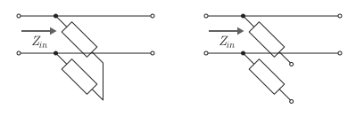
Here — input impedance of the parallel circuit. The ABCD parameters for the parallel loop are calculated as follows:
If for an argument
StubModethe value is set"Series", then the two-port network is a serial transmission line that can be closed or opened, as shown in the following figure.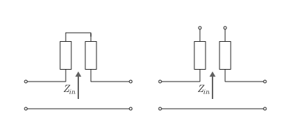
Here — input impedance of the serial circuit. The ABCD parameters for the serial loop are calculated as follows: