Optimal satellite control using the Ricatti equations
The satellite in orbit constantly deviates from its calculated trajectory: the Earth's gravity is not uniform, the Sun and Moon are pulling in different directions, and the engines are operating with an error.
The task of the control system is to keep the spacecraft in a reference orbit, minimizing fuel consumption. Fuel is mass, mass is life span. Therefore, the question "how to spend less, but keep it accurate" turns into an optimal management problem.
> **The Riccati equation is a mathematical bridge between "I want to stabilize the system" and "I want to do it with minimal cost." It gives a feedback control law of the form u = −Kx, where the gain matrix K is calculated from the solution of the Riccati equation. At the same time, you do not need to manually select the coefficients of the PID controller - they are obtained automatically and are optimal for the selected weights.
We will consider three tasks::
- Holding in a circular orbit is a classic LQR, matrices A and B are constant, the Riccati equation is solved once.
- Staying in a halo orbit near the point of the L1 matrix A(t) and B(t) periodically depend on time, and the Riccati equation must be solved for each moment of the orbit.
- Retention in nonlinear dynamics — SDRE: the Riccati equation in the control loop.
Task 1. Maintaining a circular orbit (LQR)
** What we decide.** The satellite must remain in the vicinity of a circular orbit of radius r. The model of relative motion in the orbital coordinate system (the Clohessy–Wiltshire equations) is linearized as:
where x = [δx, δy, δz, δẋ, δẏ, δż]ᵀ are deviations in position and velocity from the reference orbit, u = [uₓ, u_y, u_z]ᵀ — acceleration from the engines.
Matrices and their meaning:
A— dynamics matrix (6×6), contains gravitational terms and Coriolis accelerations;B— control matrix (6x3), shows how thrust affects speeds;Q— penalty for deviation (6×6), the larger the elementQ[i,i], the more we punish for deviation along the i-th coordinate;R— penalty for fuel consumption (3×3), the moreR, the more economical the management is;P— solution of the Riccati equation (6×6), symmetric positive-definite matrix;K = R⁻¹BᵀP— the optimal gain factor, which we apply to the law u = −Kx.
Install libraries that may not be in your system.:
Pkg.add(["ControlSystems", "DifferentialEquations"])
gr()
using ControlSystems, LinearAlgebra

# --- Orbit parameters ---
μ  = 3.986e5       # Earth's gravity parameter, km3/s2
r  = 6771.0        # the radius of the orbit, km
n  = sqrt(μ/r^3)   # average angular velocity, rad/s

# --- Clohessy–Wiltshire matrices (linearization of relative motion) ---
A = [0 0 0  1 0 0;
     0 0 0  0 1 0;
     0 0 0  0 0 1;
     3n^2 0 0  0 2n 0;
     0 0 0  -2n 0 0;
     0 0 -n^2 0 0 0]

B = [0 0 0; 0 0 0; 0 0 0; 1 0 0; 0 1 0; 0 0 1]

# --- Weights: Q punishes deviation in position more than in speed ---
# Q = diagm([1.0, 1.0, 1.0, 0.1, 0.1, 0.1])
# R = 100.0 * I(3) # expensive fuel → economical management

Q = diagm([0.01, 0.01, 0.01, 0.1, 0.1, 0.1])   # weak position penalty
R = 1e4 * I(3)                                  # expensive fuel

# --- Solve the Riccati equation and get K ---
P = care(A, B, Q, R)
K = inv(R) * B' * P

println("Optimal gain factor K:")
display(round.(K, digits=3))
println("\nСобственные числа замкнутой системы (должны быть в левой полуплоскости):")
display(round.(eigvals(A - B*K), digits=4))
Visualization. Let's run a simulation with an initial X-axis deviation and see how the satellite returns to its reference orbit.
# --- Simulation of a closed system with perturbation ---
x0 = [5.0, 0.0, 0.0, 0.0, 0.0, 0.0]
t  = range(0, stop=4000.0, length=2000)

# Open system: physics only, no regulator
sys_open = ss(A, B, Matrix(1.0I,6,6), zeros(6,3))

# Perturbation: constant acceleration along the orbit (order J2)
d_along(t) = 1e-3                       # km/s2
# and a weak sinusoid along the radial for clarity
d_rad(t)   = 3e-4 * sin(2π * t / 5400)
# The scale of the disturbance is a couple of orders of magnitude larger than usual for visualization

# The law of control + the disturbance acting at the entrance of the object
# (the controller "sees" only x, the disturbance is added as an external input)
function u_fb(x, t)
    return -K*x .+ [d_along(t), d_rad(t), 0.0]
end

res = lsim(sys_open, u_fb, t, x0=x0)
x      = res.x        # 6×2000
t_out  = res.t

# --- Control that is actually provided by the regulator (without disturbance) ---
u = -K * x
u_norm_mm = [norm(u[:, i]) for i in 1:size(u, 2)] .* 1e3

# --- Schedule ---
p1 = plot(t_out, x[1,:], label="δx (along the orbit)", lw=2,
          xlabel="time, from", ylabel="km", title="Deviation from the reference orbit (with perturbation)")
plot!(p1, t_out, x[2,:], label="δy (radial)", lw=2)
plot!(p1, t_out, x[3,:], label="δz (lateral)", lw=2)

p2 = plot(t_out, u_norm_mm, lw=2, color=:red, legend=false,
          xlabel="time, from", ylabel="мм/с²", title="Management expense ‖u‖")

plot(p1, p2, layout=(2,1), size=(800,600))
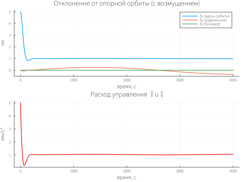
** What we see.** Constant matrix K provides a smooth return to zero in a few thousand seconds. Control is maximized at the beginning (you need to cancel the deviation), then it tends to zero. This is the optimal balance between accuracy and fuel — exactly the one that is set by the scales. Q and R.
Task 2. Maintaining a halo orbit around L1 (periodic table)
** What we decide.** In the vicinity of the Lagrange point L1 (the Sun–Earth system), there are halo orbits - periodic trajectories with a period of about six months. Here are the matrices A(t) and B(t) periodically change in time because linearization is performed at each point of the turn. The Riccati equation becomes differential:
** What does this change in practice.** Instead of a single call care we solve the inverse problem: integrate the Riccati equation backwards in time on one period and get a periodic solution. P(t). It is used to build K(t) = R⁻¹B(t)ᵀP(t), and control u(t) = −K(t)x(t) takes into account which phase of the turn the device is in.
The meaning of variables:
A(t),B(t)— linearized matrices at the current point of the halo orbit (depending on the phase of the orbit);P(t)— DRE's solution is no longer a constant, but a function of time;K(t)— periodic gain factor;- integration is carried out in reverse time from
t = Tbeforet = 0because the DRE for the stabilizing solution is a boundary value problem (boundary conditionP(T) = P(0)).
** Concise implementation of the idea.** For demonstration, we use a simple Hill model with modulation n(t) = n₀(1 + ε·cos(2πt/T)) — this is a crude but clear imitation of periodicity.:
using DifferentialEquations

T_period = 1.0                      # normalized turn period
ε = 0.3                             # modulation amplitude

# --- Periodic matrices A(t), B(t) ---
function A_t(t)
    n_t = 1.0 * (1 + ε*cos(2π*t/T_period))
    return [0 0 0  1 0 0;
            0 0 0  0 1 0;
            0 0 0  0 0 1;
            3n_t^2 0 0  0 2n_t 0;
            0 0 0  -2n_t 0 0;
            0 0 -n_t^2 0 0 0]
end
B_t(t) = [0 0 0; 0 0 0; 0 0 0; 1 0 0; 0 1 0; 0 0 1]

Q = diagm([1.0, 1.0, 1.0, 0.1, 0.1, 0.1])
R = 100.0 * I(3)

# --- DRE in reverse time: dP/dt = -(AᵀP + PA - PBR⁻1BᵀP + Q) ---
function dre!(dP, P, p, t)
    P = reshape(P, 6, 6)
    At, Bt = A_t(t), B_t(t)
    dP_mat = -(At'P + P*At - P*Bt*inv(R)*Bt'*P + Q)
    dP .= vec(dP_mat)
end

# Initial approximation: stationary solution at t=0
P0 = care(A_t(0), B_t(0), Q, R)
prob = ODEProblem(dre!, vec(P0), (T_period, 0.0))   # integrate backwards: (T, 0)
sol = solve(prob, Tsit5(), saveat=range(T_period, 0.0, length=200))

# --- Visualization: how K(t) changes along the turn ---
K_norm = [norm(inv(R)*B_t(t)'*reshape(sol(t),6,6)) for t in range(0, T_period, length=200)]
plot(range(0, T_period, length=200), K_norm, lw=2,
     xlabel="turn phase (normalized)", ylabel="‖K(t)‖",
     title="Periodic gain in halo orbit")
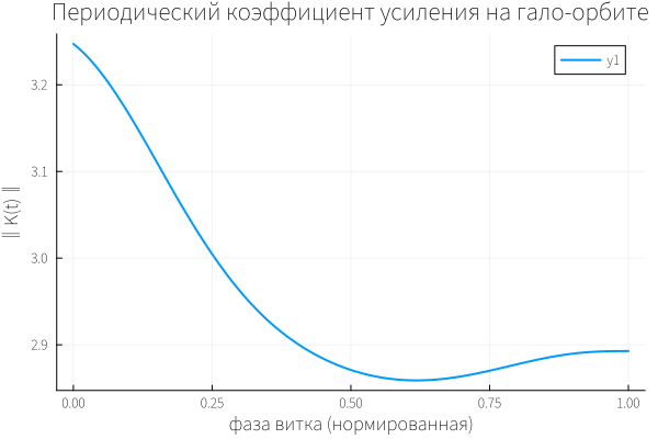
** What we see.** The norm ‖K(t)‖ it is not constant: it "breathes" along with the phase of the revolution. In the part of the orbit where the dynamics is more sensitive to disturbances, the controller becomes tougher; where the device is moving "calmly", it becomes softer. This is the advantage of the periodic approach: we do not waste fuel on excessive control in the "light" phases of the turn.
Problem 3. Nonlinear dynamics (SDRE)
In the first two examples, we used fixed matrices A and B Questioner: It was believed that the dynamics of a satellite does not depend on where it is located. For small deviations from a circular orbit, this is reasonable. But as soon as the spacecraft moves away from the reference point — for example, in an elliptical orbit or during the transition between orbits — the linearization matrices begin to depend on the current state.: A(x), B(x). Here, the usual LQR is replaced by SDRE (State-Dependent Riccati Equation): the Riccati equation is solved anew at each step, with up-to-date matrices, and the gain factor K(x) adjusts to the driving mode.
Let's make a third scenario: the same satellite, the same goal — to keep it near the reference orbit, but now A and B recalculated at each point of the trajectory. Let's see how it behaves. ‖K(t)‖ and what does it do compared to a fixed one? K.
using ControlSystems, LinearAlgebra

# --- Parameters ---
μ  = 3.986e5
r0 = 6771.0
n0 = sqrt(μ/r0^3)

# --- Plotting A(x), B(x): linearization depends on the current radius ---
# We use the Clohessy–Wiltshire model, but with n(x) = sqrt(µ/r(x)^3),
# where r(x) = r0 + δy (radial deviation)
function build_AB(x)
    r  = r0 + x[2]                 # Current radius: reference + radial deviation
    n  = sqrt(μ / r^3)             # local angular velocity
    A  = [0 0 0  1 0 0;
          0 0 0  0 1 0;
          0 0 0  0 0 1;
          3n^2 0 0  0 2n 0;
          0 0 0  -2n 0 0;
          0 0 -n^2 0 0 0]
    B  = [0 0 0; 0 0 0; 0 0 0; 1 0 0; 0 1 0; 0 0 1]
    return A, B
end

# --- Weights ---
Q = diagm([1.0, 1.0, 1.0, 0.1, 0.1, 0.1]) ./ 10
R = 100.0 * I(3) .* 10
# A multiplier of 10 has been introduced for a more visual visualization.

# --- SDRE simulation: care at every step ---
x0    = [5.0, 0.0, 0.0, 0.0, 0.0, 0.0]
t_end = 4000.0
dt    = 1.0
t_grid = 0.0:dt:t_end

x = copy(x0)
xs = zeros(6, length(t_grid))
Ks = zeros(length(t_grid))
us = zeros(3, length(t_grid))

for (i, t) in enumerate(t_grid)
    A_t, B_t = build_AB(x)
    P = care(A_t, B_t, Q, R)           # the Riccati equation in the current step
    K = inv(R) * B_t' * P
    u = -K * x
    xs[:, i] = x
    Ks[i]    = norm(K)
    us[:, i] = u
    # The integration step (explicit Euler; enough for the article)
    x = x + dt * (A_t * x + B_t * u)
end

# --- For comparison: fixed K from the reference point ---
A0, B0 = build_AB(x0)
K_fix  = inv(R) * B0' * care(A0, B0, Q, R)

x_fix = copy(x0)
xs_fix = zeros(6, length(t_grid))
for (i, t) in enumerate(t_grid)
    A_t, B_t = build_AB(x_fix)
    u = -K_fix * x_fix
    xs_fix[:, i] = x_fix
    x_fix = x_fix + dt * (A_t * x_fix + B_t * u)
end
We expect the norm to be‖K(t)‖ it will not be constant: as the satellite deviates in radius, the local angular velocity n(x) The matrix is changing A(x) It "breathes", and the SDRE controller adjusts the gain. Where the dynamics are more sensitive, K it gets tougher; where it's calmer— it gets softer.
In addition, we expect that SDRE and fixed K they will give close trajectories with small deviations (because n(x) ≈ n0), but SDRE will hold zero a little more precisely, since it "knows" about the current radius. The difference should be small, and this is also an important conclusion: SDRE is not a panacea for small deviations, but a necessity for large ones.
p1 = plot(t_grid, Ks, lw=2, color=:blue,
          xlabel="time, from", ylabel="‖K(t)‖",
          title="SDRE: The gain is recalculated at each step")
hline!(p1, [norm(K_fix)], ls=:dash, color=:gray, label="‖K‖ fixed")

p2 = plot(t_grid, xs[2,:], label="SDRE", lw=2,
          xlabel="time, from", ylabel="δy, km",
          title="Radial deviation: SDRE vs fixed K")
plot!(p2, t_grid, xs_fix[2,:], label="fixed K", lw=2, ls=:dash)

p3 = plot(t_grid, [norm(us[:,i]) for i in 1:length(t_grid)] .* 1e3,
          lw=2, color=:red, legend=false,
          xlabel="time, from", ylabel="мм/с²", title="Consumption Management (SDRE)")

plot(p1, p2, p3, layout=(3,1), size=(800,900))
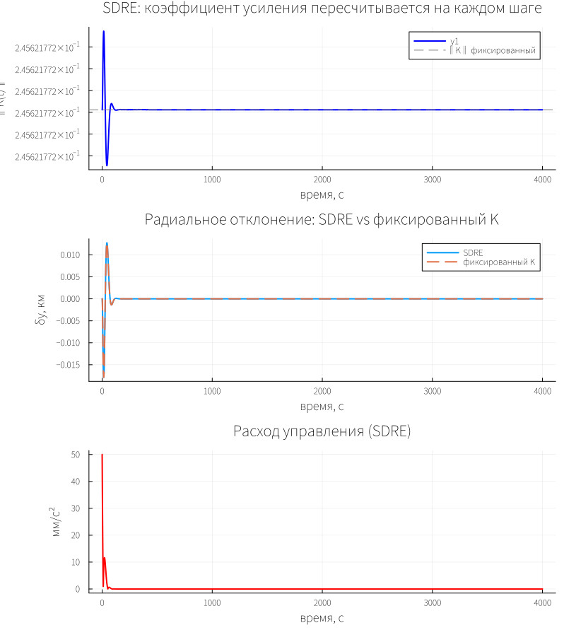
** What we see:** On the first chart ‖K(t)‖ indeed changes along the trajectory: at the beginning, while the deviation is large, the regulator is tighter; as it enters the reference orbit ‖K‖ it is approaching the value corresponding to n0. The dotted line of the fixed K it lies inside this range — SDRE "hugs" it from above and below.
In the second graph, the trajectories almost coincide: at a deviation of 5 km, the difference between the SDRE and the fixed K It's small. This is expected — n(x) it doesn't change much, yet δy ≪ r0. But if you increase the initial deviation to tens of kilometers, the SDRE will start to gain significantly: fixed K It is designed for the "wrong" angular velocity and either overshoots or undershoots.
The third graph shows that the control flow in SDRE ** is gradually decreasing** — the regulator does not "twitch" when recalculating K because the matrices change continuously along with the state.
In practice care It can be expensive for an on-board computer at each step, so approximations are used in real missions: the X-D method, small-parameter expansion, neural network surrogates for solving the Riccati equation, or precomputed tables. K(x) for typical modes, all this preserves the idea of SDRE, but removes the need to solve the Riccati equation in real time.
Conclusions
All three tasks solve the same engineering problem — ** to keep the satellite where it is needed by spending a minimum of fuel** — but with different levels of model detail.
The Riccati equation gives a formal answer to the question "how", and the matrices Q and R — to the question "at what price". By changing them, the engineer manages the compromise between accuracy and resource without rewriting the control law. In the SDRE loop, it works as a computing core that outputs an up-to-date output at each step. K(x), and this allows the regulator to remain optimal where fixed matrices no longer describe the dynamics.