Search for optimal ODE parameters
This example demonstrates the workflow for finding optimal parameters for an ordinary differential equation (ODE) describing a chain of chemical reactions. We will find the parameters and evaluate how closely they can reproduce the true dynamics of the system.
This task was solved using the [problem-oriented optimization] workflow (https://engee.com/community/catalogs/projects/algoritm-resheniia-zadach-optimizatsii ).
In this example, we will use the functions of the [JuMP.jl] library(https://engee.com/helpcenter/stable/en/julia/JuMP/index.html ) to formulate an optimization problem using the nonlinear optimization library Ipopt.jl, a library for solving differential equations DifferentialEquations.jl and the [Plots.jl] library(https://engee.com/helpcenter/stable/en/julia/juliaplots/index.html ) to visualize the results.
Task description
Let's consider a model of a multi-stage chain of chemical reactions involving several substances. . Substances react with each other at a certain rate and they form new substances. The true reaction rate for this task is unknown. But we can make observations a certain number of times in a given time. . Based on these observations, we will select the optimal reaction rates. .
There are six substances in the model, from before which react as follows:
- one substance and one substance they react to form a single substance with speed ;
- one substance and one substance they react to form a single substance with speed ;
- one substance and one substance they react to form a single substance with speed .
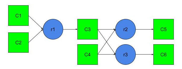
The reaction rate is proportional to the product of the quantities of the required substances. Thus, if represents the amount of substance , then the reaction rate to obtain equal to . Similarly, the reaction rate to obtain equal to , and the reaction rate to obtain equal to .
Thus, we can create a differential equation describing the process of changing our system.:
Setting the initial values . Such initial values ensure that all substances fully react, resulting in they will approach zero as the time increases.
Installing Libraries
If the latest version of the package is not installed in your environment JuMP, uncomment and run the cell below:
Pkg.add(["Ipopt", "DifferentialEquations", "JuMP"])
# Pkg.add("JuMP");
To launch a new version of the library after the installation is complete, click on the "Personal Account" button:
 Then click on the "Stop" button:

Restart the session by clicking the "Start Engee" button:

Connecting libraries
Connect the library JuMP:
using JuMP;
Connect the library of the nonlinear solver Ipopt:
using Ipopt;
Connect the library to solve differential equations DifferentialEquations:
using DifferentialEquations;
Connect the charting library Plots:
using Plots;
Configuration of visualization parameters
Set a customized chart size and background plotly:
plotly(size=(1500, 600), xlims=(0, :auto));
Describe the function that defines the boundaries for and axes for approximating graphs:
function check_bounds(min::Number, max::Number)
    if min > max
        error("The min value must be less than the max value.")
    elseif max < min
        error("The max value must be greater than the min value.")
    end
end
Solving differential equations
Create a function dif_fun, describing an ODE to our chain of chemical reactions:
function dif_fun(du, u, p, t)
    r1, r2, r3 = p

    du[1] = -r1 * u[1] * u[2]
    du[2] = -r1 * u[1] * u[2]
    du[3] = -r2 * u[3] * u[4] + r1 * u[1] * u[2]- r3 * u[3] * u[4]
    du[4] = -r2 * u[3] * u[4] - r3 * u[3] * u[4]
    du[5] = r2 * u[3] * u[4]
    du[6] = r3 * u[3] * u[4]
end
Set the true values and save them in a variable. r_true:
r_true = [2.5, 1.2, 0.45];
Values , and in the variable r_true they are the benchmark that the optimization algorithm should try to recreate.
Set the duration of the reaction simulation and the initial values for :
t_span = (0.0, 5.0);
y_0 = [1.0, 1.0, 0.0, 1.0, 0.0, 0.0];
Create an ODE task using the function ODEProblem:
prob = ODEProblem(dif_fun, y_0, t_span, r_true);
Solve the problem using the function solve. In parentheses, specify the name of the solver and the frequency of observations in the argument. saveat:
sol_true = solve(prob, Tsit5(), saveat=0.1);
To solve this problem, we use the Runge-Kutta Tsipouras solver of the 5th order. Tsit5(), which is рекомендованным for most non-rigid tasks.
Display the results of the true solutions on graphs:
colors = [:red, :blue, :green, :orange, :purple, :brown]

plot(layout=(3,2))
for i in 1:6
    plot!(subplot=i, sol_true.t, sol_true[i,:], color=colors[i], title="y($i)", label="True y($i)")
end
display(current())
Solving the optimization problem
Describe the objective function obj_fun, calculating the difference between the true parameters , and and calculated values.
function obj_fun(r1, r2, r3)
    r = [r1, r2, r3]
    prob_new = ODEProblem(dif_fun, y_0, t_span, r)
    sol_new = solve(prob_new, Tsit5(), saveat=0.1)
    return sum(sum((sol_new[i,:] .- sol_true[i,:]).^2) for i in 1:6)
end
To find optimal solutions, we will need to minimize this function.
Create an optimization task using the function Model and specify the name of the solver in parentheses.:
model = Model(Ipopt.Optimizer)
Switch the model to silent mode to hide system messages.:
set_silent(model)
Create a variable r containing three elements – , and , and set the bounds from 0.1 to 10:
@variable(model, 0.1 <= r[1:3] <= 10)
Since we are dealing with a complex user-defined nonlinear function obj_fun, for proper integration into the library's optimization environment JuMP it must first be registered using the function register. Specify the number of incoming arguments in parentheses (, and ) and enable automatic differentiation.
register(model, :obj_fun, 3, obj_fun; autodiff = true)
Create a non-linear objective function to find the minimum values. , and and apply the previously created function obj_fun:
@NLobjective(model, Min, obj_fun(r[1], r[2], r[3]))
Solve the optimization problem:
optimize!(model);
Save the optimized parameters in a variable:
optimized_params = value.(r)
Print the results of solving the problem. You can use the function round and the argument digits to adjust the accuracy to the accuracy of the true parameter data.
optimized_params = round.(value.(r), digits=2)
println("True parameters: ", r_true)
println("Optimized parameters: ", optimized_params)
Optimization with limited observations
Let's model a situation where we can't observe all the components. , but only the final results and , and calculate the values of the rates of all reactions based on this limited information.
Describe the objective function obj_fun_lim, which is a copy of the function obj_fun from the previous section, but returning only the results for and .
function obj_fun_lim(r1, r2, r3)
    r = [r1, r2, r3]
    prob_new = ODEProblem(dif_fun, y_0, t_span, r)
    sol_new = solve(prob_new, Tsit5(), saveat=0.1)
    return sum(sum((sol_new[i,:] .- sol_true[i,:]).^2) for i in 5:6)
end
Create an optimization task using the function Model and specify the name of the solver in parentheses.:
model_lim = Model(Ipopt.Optimizer)
Switch the model to silent mode to hide system messages.:
set_silent(model_lim)
Create a variable r containing three elements – , and , and set the bounds from 0.1 to 10:
@variable(model_lim, 0.1 <= r_lim[1:3] <= 10)
Register the function obj_fun_lim using the function register:
register(model_lim, :obj_fun_lim, 3, obj_fun_lim; autodiff = true)
Create a non-linear objective function to find the minimum values. , and and apply the previously created function obj_fun_lim:
@NLobjective(model_lim, Min, obj_fun_lim(r[1], r[2], r[3]))
Solve the optimization problem:
optimize!(model_lim)
Print the results of solving the problem. You can use the function round to round up overly precise values, if necessary.
println("True parameters: ", r_true)
println("Optimized parameters (limited): ", value.(r_lim))
Create an ODE task using the function ODEProblem by applying optimized values r_lim:
prob_opt = ODEProblem(dif_fun, y_0, t_span, value.(r_lim));
Solve the ODE problem:
sol_opt = solve(prob_opt, Tsit5(), saveat=0.1);
Visualize the results for and :
y_min = 0 # @param {type:"slider", min:0, max:1, step:0.01}
y_max = 0.6 # @param {type:"slider", min:0, max:1, step:0.01}
check_bounds(y_min, y_max)
x_min = 0 # @param {type:"slider", min:0, max:5, step:0.1}
x_max = 5 # @param {type:"slider", min:0, max:5, step:0.1}
check_bounds(x_min, x_max)

plot(sol_true.t, [sol_true[5,:] sol_true[6,:]], label=["True y(5)" "True y(6)"], ylimits=(y_min, y_max), xlimits=(x_min, x_max))
plot!(sol_true.t, [sol_opt[5,:] sol_opt[6,:]], label=["Optimized y(5)" "Optimized y(6)"], linestyle=:dash, ylimits=(y_min, y_max), xlimits=(x_min, x_max))
display(current())
Visualize and compare the results of the previously set true values and the obtained values. :
true_colors = [:darkred, :darkblue, :darkgreen, :darkorange, :darkviolet, :brown]
opt_colors = [:red, :blue, :green, :orange, :violet, :orange]

plot(layout=(3,2))
for i in 1:6
    plot!(subplot=i, sol_true.t, sol_true[i,:], color=true_colors[i], label="True y($i)", title="y($i)")
    plot!(subplot=i, sol_opt.t, sol_opt[i,:], color=opt_colors[i], label="Optimized y($i)", linestyle=:dash)
end
display(current())
We can find that with the new optimized parameters obtained with limited observations, substances and they are consumed more slowly, and the substance accumulates to a lesser extent. However, the substances , and they have exactly the same dynamics for both found and true parameters.
Conclusion
In this example, we solved the problem of finding optimal parameters of an ODE describing a multi-stage chain of chemical reactions using the workflow [problem-oriented optimization] (https://engee.com/community/catalogs/projects/algoritm-resheniia-zadach-optimizatsii ). We modeled the situation with limited observations and compared the dynamics of the system.