Graphical representation of sparse matrices
In this example, we will create a grid for calculating the final elements of the NASA airfoil - a wing and two flaps. We will run the resulting graph through different algorithms to show how the representation of the adjacency matrix of the graph can be optimized.
Uploading data
For further work, we will need libraries for graph visualization, special functions from the SparseArrays library (written in C and optimized), as well as two function libraries written in Julia.
Pkg.add( ["Graphs", "GraphPlot", "AMD", "SymRCM"] )
The data is stored in a file airfoil.jld2 and contain:
- 4253 pairs of coordinates (x,y) of grid points
- An array of 12,289 pairs of indexes (i,j) defining connections between grid points
Upload the data file to the workspace.
using FileIO
i,j,x,y = load( "$(@__DIR__)/airfoil.jld2", "i", "j", "x", "y" );
Visualization of a finite element grid
Let's create a sparse adjacency matrix from the connection vector (i,j) and make it positive definite. Then we plot the adjacency matrix using (x,y) as the coordinates of the vertices (grid points).
For additional acceleration, we instruct the system to save graphs in PNG format and not use interactive visualization.
gr( fmt = "png", size=(600,400) );
using SparseArrays, Graphs, GraphPlot
n = convert(Int32, max( maximum(i), maximum(j) ));
A = sparse( vec(i), vec(j), -1.0, n, n );
A = A .+ A';
gplot( Graph( A ), vec(x), .-vec(y), EDGELINEWIDTH=0.3,
edgestrokec = "deepskyblue", nodefillc = "deepskyblue",
plot_size = (16cm, 12cm), title="Wing and flap profile" )
Visualization of the adjacency matrix
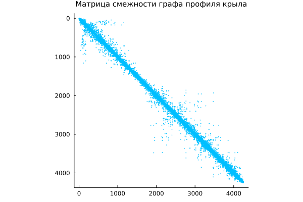
Function spy It allows you to visualize nonzero matrix elements, which is especially useful for analyzing the structure of sparse matrices. spy(A) displays the structure of the nonzero elements of the matrix A.
spy( A, c="deepskyblue",
title="The adjacency matrix of the wing profile graph",
titlefont=font(10) )
Symmetric reordering is the inverse of the Cuthill-McKee algorithm
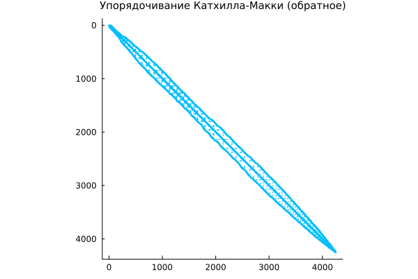
The Cuthill—McKee algorithm renumbers the vertices of a graph so that its adjacency matrix (which we are studying) has the smallest ribbon width. The reverse algorithm (RCM, reverse Cuthill—McKee) simply numbers the vertex indexes in the opposite direction.
Algorithms for RCM appeared a long time ago, and you can use an older implementation in the [CurthillMcKee.jl] package(https://github.com/rleegates/CuthillMcKee.jl ).
symrcm implements the inverse Cuthill-McKee transformation for rearranging the adjacency matrix. Team r = symrcm(A) returns the permutation vector r, in which the matrix A[r,r] It has diagonal elements located closer to the main diagonal than in the original matrix A.
using SymRCM
r = symrcm(A)
spy( A[r,r], c="deepskyblue",
title="The Cuthill-McKee ordering (reverse)",
titlefont=font(10) )
This format is useful as a pre-ordering for LU factorization or Cholesky decomposition. It works for both symmetric and non-symmetric matrices.
The original adjacency matrix may have non-zeroes "smeared" over its entire area. The RCM permutation arranges the points so that the non-zeroes are concentrated at the diagonal, after which calculations can be performed more efficiently.
Symmetric reordering - rearranging columns
Julia does not have a default function for obtaining a permutation vector that orders the columns of a sparse matrix. A in the order of non-decreasing number of non-zero elements. This approach is also sometimes useful as a pre-ordering for LU decomposition, for example lu(A[:,j]).
Because the essence of the operation is colperm extremely simple, it's easier to write your own implementation.:
function colperm(S::SparseMatrixCSC)
nnz_per_col = sum(S .!= 0, dims=1) # The number of non-zero elements in each column
return sortperm(vec(nnz_per_col)) # Returns a permutation of indexes
end
j = colperm( A )
spy( A[j,j], c="deepskyblue",
title="Ordering by the number of items in columns",
titlefont=font(10) )
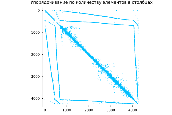
This operation allows for more efficient matrix compression, and can also reduce the number of nonzero elements generated by the LU decomposition commands.
Symmetric approximate minimum order
Team amd performs a symmetric permutation using the approximate minimum order method from the corresponding package. For a symmetric positive definite matrix A team p = amd(A) returns the permutation vector p, in which the matrix A[p,p] has a more sparse Cholesky multiplier than the original one A. Sometimes amd It also works well for symmetric indefinite matrices.
using AMD
m = amd(A);
spy( A[m,m], c="deepskyblue",
title="Approximate minimum order",
titlefont=font(10) )
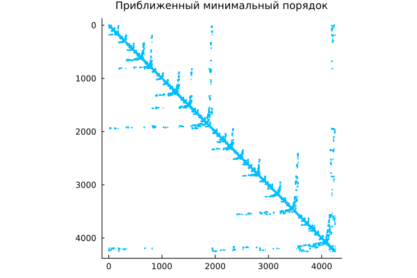
Again, we find a permutation in which subsequent decomposition algorithms introduce fewer new nonzeros, while maintaining symmetry (important for problems in mechanics and physics).
Conclusion
All these algorithms help to prepare data for faster and more stable solutions to the weaknesses that arise in wing strength calculations, aerodynamic modeling, thermal analysis, etc. By applying optimization, we will most likely be able to reduce the time needed to solve the problem by 2-3 orders of magnitude.
Additional algorithms are available, for example, in packages Metis.jl and IterativeSolvers.jl. The first contains algorithms for graph reordering, the second contains additional methods for working with sparse matrices. We also recommend that you study SuiteSparse - a wrapper over well-tested industrial C code, but it lacks some of the features that we needed.