Finding the shortest path on a graph
In this example, we will use the library functions. Graphs.jl to create a graph and find the shortest route between two points on it.
Working with graphs
Graphs are often used as an element of models in logistics, transportation, information, or social media tasks, and other related systems. They are abstract mathematical objects consisting of vertices (vertex, vertices) and edges (edges). Usually, each vertex has its own unique number, and the edges are indicated by two numbers – the numbers of the vertices they connect.
Some information may be associated with nodes and edges (for example, coordinates or bandwidth). In the library Graphs.jl it is assumed that additional information is stored in an external table or dictionary (Dict). Records can be linked to vertices (via their numbers) or edges (via a tuple of numbers identifying the edge). Sparse matrices can be used to save money (SparseArrays.jl).
Pkg.add(["GraphRecipes", "Graphs"])
# If you have the library installed, comment on the following line:
import Pkg; Pkg.add( ["Graphs", "GraphRecipes"] )
using Graphs, GraphRecipes
Package GraphsRecipes.jl is responsible for drawing graphs.
Let's create a simple directed graph containing three nodes and several edges.
g = DiGraph()
add_vertices!( g, 3 );
Now there are three vertices in our graph, connect them with edges.
add_edge!( g, 1, 2 );
add_edge!( g, 1, 3 );
add_edge!( g, 2, 3 );
And we will output this graph:
gr() # Simplified rendering
graphplot( g, names=1:nv(g) )
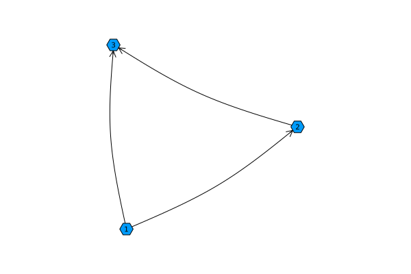
Note that the node names are names taken from an "external" array 1:nv(g) where are the node numbers stored from 1 before nv (number of vertices, the number of vertices).
Let's create a map on which we will look for a way
As a field for finding the shortest path, we will take a random matrix and set a goal to walk along it along the main diagonal. The connectivity of this "map" and the ability to reach point B from point A, alas, is not provided by anything other than choosing the "correct" starting value of the pseudorandom number generator. Random.seed!().
using Random;
Random.seed!( 4 )
map = rand( 30, 30 ) .> 0.3;
heatmap( map )
# The starting and finishing point
DOT_A = CartesianIndex(1,1)
DOT_B = CartesianIndex(30,30)
# Let's add the start and finish currents to the graph.
scatter!( [DOT_A[1]], [dot_a[2]], c=:red )
scatter!( [DOT_B[1]], [dot_b[2]], c=:green, leg=false )
Our graph will be undirected, that is, along each edge it will be possible to go both there and back.
g = Graph();
indexes of available points = LinearIndices( map )[ the map .== 1 ]
println( "The number of platforms where you can step on: ", count(индексы_доступных_точек .> 0 ))
Auxiliary objects (coordinate translation)
Let's save the matrix where the 2D coordinates of all points on the map will be stored.
coordinates of all points = CartesianIndices( size(map) );
Let's create a graph that translates the vertex number of the graph into a coordinate:
point coordinates of the graph = Dict(zip( 1:length(indexes of available points), coordinates of all points[indexes of available points] ))
first( sort(collect(point_graph coordinates)), 5 )
Now we invert this dictionary and get the opportunity to translate a coordinate into a point number on the graph.
point_points by coordinates = Dict(value => key for (key, value) in point_graph coordinates)
first( sort(collect(point_ indexes by coordinates)), 5 )
Add the coordinates of the points into arrays xx and yy – we will transfer them to the graph rendering procedure.
xy = Tuple.(first.(sort(collect(point_ indexes by coordinates))));
xx = first.(xy);
yy = last.(xy);
Filling the graph
Since we will use the standard function to find the shortest path, rather than creating it ourselves from scratch, we need to create a graph on which this search will take place.
g = Graph()
add_vertices!( g, length(coordinates of all points[ indexes of available points ][:]) )
Let's go through all the points and connect them with neighboring points, if there is a passage between them.
MAX_X,MAX_Y = size(map )
for vertex in 1:nv(g)
x,y = Tuple(point coordinates of the graph[vertex])
right_point = CartesianIndex( x + 1, y )
point_side = CartesianIndex( x, y + 1 )
# Connect the current point to the point on the right, if there is a connection according to the map of passed points.
if x < MAX_X && map[access point] == 1 add_edge!(g, vertex, point_indication_coordinates[right_point]); end;
# The same is true for the point from below
if y < MAX_Y && map[point down] == 1 add_edge!(g, vertex, point_indexs_coordinates[point_side]); end;
end
Let's see if any edges have been added to our graph, and how many of them there are:
g
Judging by the output, 840 edges were added to 634 points. Let's output a graph:
heatmap( карта', title="Map", titlefont=font(9), leg=:false )
graphplot!( g, x = xx, y = yy, nodeshape=:circle, nodecolor=:red, nodestrokecolor=:red, nodesize=1.5, edgecolor=:red, curves=true, size=(500,500) )
We didn't have to "lay out" the graph, because we already know the coordinates of each node. The rest of the rendering parameters can be studied [here] (https://juliagraphs.org/GraphPlot.jl /).
Finding the shortest path
We use the [A-star algorithm](https://juliagraphs.org/Graphs.jl/dev/algorithms/shortestpaths /), which searches for the shortest path using heuristics. At the output, we get a set of edges.
# Finding the shortest path
path = a_star( g, indexes point to coordinates[point A], indexes point to coordinates[point B] );
first( path, 5 )
Let's make an array of graph points that need to be visited to go from point A to point B.
points = Tuple.( vcat([point A], [ point coordinates[dst(v)] for v in path ]) );
first( points, 5 )
# Map output (with offset values for the desired graph brightness)
heatmap( карта' .* 0.3 .+ 0.7, title="The shortest path", leg=false, c=:grays, aspect_ratio=:equal )
# Output of a graph of acceptable movements on the map
# graphplot!( g, x = xx, y = yy, curves=true, nodeshape=:circle, size=(400,400) )
# Deducing the shortest path
plot!( first.(points), last.(points), lw=3, linez=range(0,1,length(points)), c=:viridis, yflip=true )
Conclusion
Graphs are very powerful mathematical objects that allow you to find structure in disparate data–cycles, trees, shortest or longest paths, and connected regions. The opportunity to work with them from a dynamic systems modeling environment gives engineers very interesting opportunities.