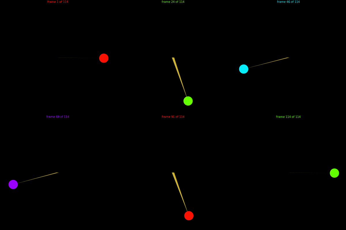
Animation of the movement of a pendulum using Julia

This example shows the implementation of simulating the movement of a physical pendulum using differential equations and creating animations in the Julia programming language.

Introduction

A pendulum is the simplest physical system widely used to study periodic motion and oscillations. In this example, we consider the problem of modeling the motion of a simple pendulum using a system of second-order ordinary differential equations, which is then solved in the framework of a boundary value problem using the collocation method (MIRK). After finding a solution, it is visualized in GIF animation format using the Luxor.jl library based on Cairo.

The main goal is to demonstrate the capabilities of the Julia language in numerical solution of physical problems and generation of graphical visualization. Animation allows you to understand the dynamics of a pendulum's movement — how it moves over time, starting from a given position and ending at the opposite point after a certain time interval.

# Installing required packages
import Pkg; Pkg.add("Luxor")
import Pkg; Pkg.add("Colors")
import Pkg; Pkg.add("BoundaryValueDiffEq")

Connecting libraries

using Luxor        # for drawing animations
using Colors       # to control the colors of animation elements
using BoundaryValueDiffEq  # for solving boundary value problems of ordinary differential equations

Defining constants and parameters for the model

Constants of the physical model and animation

const g = 9.81;     # acceleration of gravity (m/s2)
const L = 1.0;      # length of the pendulum thread (meters)
const bobd = 0.10;  # diameter of the weight (bob) of the pendulum (in meters)

Animation Parameters

const framerate = 50.0;                # animation frame rate (fps)
const t_0 = 0.0;                        # initial simulation time (seconds)
const tf = 2.3;                        # end simulation time (seconds)
const dtframe = 1.0/framerate;         # duration of 1 frame in seconds
const tspan = LinRange(t_0, tf, Int(floor(tf*framerate)));  # an array of time points for animation

Colors and file names

const bgcolor = "black";               # animation background color
const leaderhue = (0.80, 0.70, 0.20);  # light gold color for the lever
const hslcolors = [HSL(col) for col in (distinguishable_colors(
                   Int(floor(tf*framerate)+3),[RGB(1,1,1)])[2:end])];  # a set of colors for the elements
const giffilename = "pendulum.gif";    # the name of the output GIF file

Formulation of the problem and solution of the differential equation

Definition of a function for the equations of motion of a pendulum

function simplependulum(du, u, p, t)
    θ = u[1]   # angle of deviation
    dθ = u[2]  # rate of change of angle (angular velocity)
    
    du[1] = dθ                     # derivative of the angle = angular velocity
    du[2] = -(g/L) * sin(θ)        # equation of motion: θ" = -(g/L) * sin(θ)
end

simplependulum (generic function with 1 method)

Setting boundary conditions

function bc2(residual, u, p, t)
    residual[1] = u[end÷2][1] + pi/2     # the value of the angle in the middle of the interval is equal to π/2 (position on the left)
    residual[2] = u[end][1] - pi/2       # the angle value at the end is -π/2 (position on the right)
end

bc2 (generic function with 1 method)

Formation and solution of the boundary value problem

bvp2 = BVProblem(simplependulum, bc2, [pi/2, pi/2], (tspan[1], tspan[end]));
sol2 = solve(bvp2, MIRK4(), dt=dtframe);   # the Runge–Kutta method of the 4th order with correction

Animation rendering functions

Background function for rendering a frame

function backdrop(scene, framenumber)
    background(bgcolor)   # setting the black background
end

backdrop (generic function with 1 method)

The main function of drawing each frame is

function anim_frame(scene, framenumber)
    # We get the current values of the angle and angular velocity
    u1, u2 = sol2.u[framenumber]
    # We calculate the coordinates of the bob's center using trigonometry formulas
    y = L * cos(u1)
    x = L * sin(u1)
    
    # Draw a lever (from the suspension point to the load)
    sethue(leaderhue)
    poly([Point(-4.0, 0.0), Point(4.0, 0.0),
          Point(160.0x, 160.0y)], :fill)
    
    # Draw the weight (bob) of the pendulum
    sethue(Colors.HSV(framenumber*4.0, 1, 1))  # changing color depending on the frame number
    circle(Point(160.0x, 160.0y), 160*bobd, :fill)

    # Print information about the current frame
    Luxor.text(string("frame $framenumber of $(scene.framerange.stop)"),
         Point(0.0, -190.0), halign=:center)
end

anim_frame (generic function with 1 method)

Creating and playing animations

Creating an animation object with the specified window size

muv = Movie(400, 400, "Pendulum Demo", 1:length(tspan))

Movie(400.0, 400.0, "Pendulum Demo", 1:114)

Adding two scenes: the background and the main one

Luxor.animate(muv, [
    Luxor.Scene(muv, backdrop),             # background scene
    Luxor.Scene(muv, anim_frame, easingfunction=easeinoutcubic)  # the main stage with a smooth transition
], creategif=true, pathname=joinpath(@__DIR__, giffilename))            # creating it .gif and save it under the name "pendulum.gif "

┌ Info: Frames for animation "Pendulum Demo" are being stored in directory: 
└ 	 /tmp/jl_1cbAyz
┌ Info: ... 114 frames saved in directory:
└ 	 /tmp/jl_1cbAyz
[ Info: GIF is: /user/animate_a_pendulum/pendulum.gif

Conclusion

We have reviewed a program in the Julia language that solves a boundary value problem for a pendulum motion model and builds a smooth animation in GIF format based on it. Key elements: physical model (equations of motion), numerical solution (MIRK4 method), and visualization (using Luxor). This approach is useful not only for educational purposes, but also for modeling more complex systems with constraints on initial or final conditions. This example illustrates the powerful tools in scientific computing and graphical visualization in the Julia ecosystem.

The example was developed using materials from Rosetta Code