Solving a system of differential equations under various initial conditions

In this example, we consider two approaches to solving a differential equation under different initial conditions: 1.
using a loop for with the change of n.o.
2. using EnsembleProblem for multithreaded solutions

Task description

As a test, consider the [Lotka-Volterra] equation (https://ru.wikipedia.org/wiki/Model_lotki_—_Volterra), describing the predator-prey model:

where
and - populations of prey and predator, respectively

- time

- constant parameters describing the interaction between representatives of the species.

For the sake of certainty, let's take them as equal .

In the given task, the n.o. is the size of the species population. By solving the problem, we will be able to observe the population change over time.

Let's look at which packages are needed to solve our problem.:

OrdinaryDiffEq - a package that allows you to solve ordinary problems, which can work without connecting the package DifferentialEquations
Plots It has the ability to display the solution of a differential equation in just one line.
Distributed allows you to place functions on different processor cores to increase computing efficiency.

Pkg.add(["DifferentialEquations", "OrdinaryDiffEq", "Distributed", "BenchmarkTools"])

using OrdinaryDiffEq, Plots

An ordinary d.u. has the form

To solve the problem, it is necessary to determine the following initial data:

f - the function itself (the structure of the device)

u0 - initial conditions

tspan - the time period during which a solution is sought

p - system parameters that also determine its appearance

kwargs - keywords passed to the solution

There are two ways to set the function f:

f(du,u,p,t) - memory-efficient, but may not be supported by [packages](https://fluxml.ai/Zygote .jl/dev/limitations/#Array-mutation-1), in which [mutation] is prohibited(https://docs.julialang.org/en/v1/manual/variables/#man-assignment-expressions )
f(u,p,t) - returns du. Applicable in packages where mutation is prohibited.

function lotka(du, u, p, t) 
    du[1] = p[1] * u[1] - p[2] * u[1] * u[2]
    du[2] = p[4] * u[1] * u[2] - p[3] * u[2]  
end
α = 1; β = 0.01; γ = 1; δ = 0.02;
p = [α, β, γ, δ]
tspan = (0.0, 6.5)
u0 = [50; 50]
prob = ODEProblem(lotka, u0, tspan, p)

ODEProblem with uType Vector{Int64} and tType Float64. In-place: true
timespan: (0.0, 6.5)
u0: 2-element Vector{Int64}:
 50
 50

After we have set the task, we will proceed to its solution. Function solve allows you to solve the problem using various solvers (solver). In our case, we have an ODE that can be solved with a constant step. The set problem and solver will be passed as parameters. Tsit5() and the parameter saveat=0.01, indicating to the function the step with which to save the solution.

sol = solve(prob, Tsit5(), saveat=0.01)

retcode: Success
Interpolation: 1st order linear
t: 651-element Vector{Float64}:
 0.0
 0.01
 0.02
 0.03
 0.04
 0.05
 0.06
 0.07
 0.08
 0.09
 0.1
 0.11
 0.12
 ⋮
 6.39
 6.4
 6.41
 6.42
 6.43
 6.44
 6.45
 6.46
 6.47
 6.48
 6.49
 6.5
u: 651-element Vector{Vector{Float64}}:
 [50.0, 50.0]
 [50.25062391161723, 50.00125211549466]
 [50.50249138370918, 50.00501692739517]
 [50.755595782113325, 50.01130738411668]
 [51.009930152636706, 50.020136767794746]
 [51.26548722105585, 50.031518694285374]
 [51.52225939311683, 50.04546711316499]
 [51.78023875453521, 50.06199630773043]
 [52.039417070996095, 50.081120894998996]
 [52.29978578815409, 50.10285582570839]
 [52.56133603163334, 50.127216384316746]
 [52.82405860702751, 50.15421818900265]
 [53.08794399989971, 50.18387719166507]
 ⋮
 [47.63881663670754, 50.10217268569618]
 [47.877146554422595, 50.07972805051839]
 [48.11676888713707, 50.05968794764736]
 [48.35768016469967, 50.04206191833404]
 [48.59987678709717, 50.026859716639514]
 [48.84335502445415, 50.01409130943499]
 [49.08811101703379, 50.00376687640185]
 [49.33414077523645, 49.99589681003162]
 [49.581440179601316, 49.99049171562596]
 [49.83000498080491, 49.98756241129669]
 [50.07983079966195, 49.98711992796579]
 [50.33091312712557, 49.98917550936536]

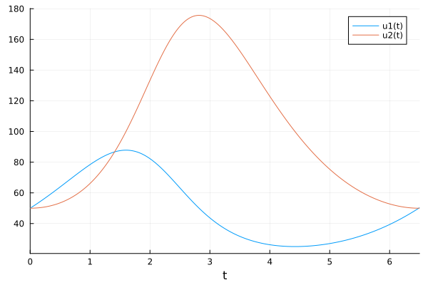
Now let's display our solution, with the legend and axis caption automatically specified. t

plot(sol)

Now let's display the phase trajectory - the change in phase coordinates (x and y) from time to time. In the figure, the initial positions are in shades of red, and at the end of the solution are blue.

scatter(
sol[1, :], sol[2, :],                           # x и y
legend=false, marker_z=sol.t, color=:RdYlBu,    # marker_z позволяет изменять цвет маркера от t
xlabel="Жертва x", ylabel="Хищник y",           # RdYlBu - от Красного до Синего через Жёлтый
title="Фазовая траектория системы")

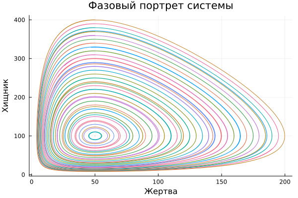
Now that we have been able to depict the phase trajectory for one pair of vehicles, we will build a phase portrait of the totality of these trajectories.

To do this, we will use a loop for gradually increasing the initial size of the predator's population.

tspan=(0., 15.)
initial_conditions = range(10, stop=400, length=40)

10.0:10.0:400.0

plt = plot()
for y0 in initial_conditions
    u0 = [50; y0]
    prob = ODEProblem(lotka, u0, tspan, p)
    sol = solve(prob, Tsit5(), saveat=0.01)
    plot!(plt, sol[1, :], sol[2, :], title="Фазовый портрет системы", xlabel="Жертва", ylabel="Хищник" ,legend=false)
end

display(plt)

Multithreaded phase portrait construction

Now let's consider another solution to the problem of constructing a phase portrait. To do this, we will connect the standard package Distributed, which allows you to perform tasks in a distributed manner. And we will distribute our task into 4 threads (processes).

using Distributed
N_PROCS = 4  # зададим количество процессов
addprocs(N_PROCS)

4-element Vector{Int64}:
 2
 3
 4
 5

By enabling DifferentialEquations - a package for solving various types of problems, we will use the function EnsembleProb, which allows you to set a change in the initial conditions by calling the function prob_func.

For example, you can change the initial conditions randomly.:

function prob_func(prob, i, repeat) 
@. prob.u0 = randn() * prob.u0 prob
end

or use an external data container:

function prob_func(prob, i, repeat)

    remake(prob, u0=[50, initial_conditions[i]])

end

using DifferentialEquations
u0 = [50; 10];
prob = ODEProblem(lotka, u0, tspan, p);

function prob_func(prob, i, repeat)
    remake(prob, u0=[50, initial_conditions[i]])
end
ensemble_prob = EnsembleProblem(prob, prob_func=prob_func)

EnsembleProblem with problem ODEProblem

Having set the task, we get a solution using solve. But this time, we will get back not just one solution, but a whole set of simulations. sim. Note that in solve added arguments:

EnsembleThreads() - meaning that the distribution will be across processor threads, rather than, for example, across different cluster computers
trajectories=N_TRAJECTS - the number of simulations we want to run

N_TRAJECTS = length(initial_conditions)
sim = solve(ensemble_prob, Tsit5(), EnsembleThreads(), trajectories=N_TRAJECTS, saveat=0.01);

Let's draw a phase portrait, going through each solution in the simulation set.

plt = plot()
for sol in sim.u
    plot!(plt, sol[1, :], sol[2, :],  title="Фазовый портрет системы", xlabel="Жертва", ylabel="Хищник" ,legend=false)
end

display(plt)

Comparison of execution time

Now let's compare the code execution time in a loop and using multithreading.

To do this, connect the library BenchmarkTools. let's set our functions that we want to compare, and use a macro @btime our functions will be run several times and their average execution time will be calculated.

using BenchmarkTools

function for_loop_solution()
    for y0 in range(10, stop=400, length=20)
        u0 = [50; y0]
        prob = ODEProblem(lotka, u0, tspan, p)
        solve(prob, Tsit5(), saveat=0.01)
    end
end

function ensemble_prob_solution()
    prob = ODEProblem(lotka, u0, tspan, p)

    initial_conditions = range(10, stop=400, length=20)
     function prob_func(prob, i, repeat)
        remake(prob, u0=[50, initial_conditions[i]])
    end
    ensemble_prob = EnsembleProblem(prob, prob_func=prob_func)
    solve(ensemble_prob, Tsit5(), EnsembleThreads(), trajectories=20, saveat=0.01)
end

@btime for_loop_solution()
@btime ensemble_prob_solution()
[];  #заглушка чтобы не выводить EnsembleProblem в ячейку вывода

  8.418 ms (33260 allocations: 3.59 MiB)
  1.869 ms (31424 allocations: 3.53 MiB)

Conclusion

Based on the results of the estimated execution time, ensemble_prob_solution it turned out to be 4 times faster, which corresponds to the number of cores allocated for the task.

From which it can be concluded that when solving a system of differential equations with different initial conditions, the cycle for it is worth preferring EnsemleProblem and distributed computing, using the package Distributed.