Distribution of a random variable in different coordinate systems
The following topics will be covered in this example:
- random number and array generation in Julia
- using probability distributions
- the importance of choosing the right distribution of a random variable depending on the problem statement.
Default random number generation
function rand()
In order to generate a random number, you can use the function without connecting libraries. rand() . It will return a random real number in the range [0,1)
Pkg.add(["Distributions"])
rand()
If you need to create a matrix a certain size with elements , then we will use rand(i,j,k)
rand(2,4,3)
If in rand() transfer a tuple:
rand((2,4,3)),
that (2,4,3) there will be a set of elements from which a random element is selected
rand((2,4,3))
rand(('a',3,"string",1+1im),2,3)
You can also pass a dictionary as a set of elements.:
rand(Dict("pi" => 3.14, "e" => 2.71), 3)
Visual analysis of the distribution
In order to visually assess the law by which numbers are generated, we will use the library Plots. To do this, connect it using using Plots and after that we will use the function histogram. By writing gr() - disable the possibility of interactive interaction with charts.
using Plots # connecting the library
gr() # disabling interactive interaction with the graph, because there are many points.
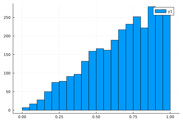
histogram(rand(50000)) # building a histogram
title!("rand(50000)") # signature
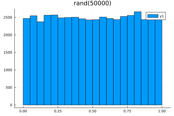
As can be seen from the histogram, the distribution of random numbers generated using rand() is uniform. That is, the function rand() generates values with standard continuous uniform distribution (SNR)
Normal distribution
Also, without connecting other libraries, Julia can generate random numbers with a normal distribution.
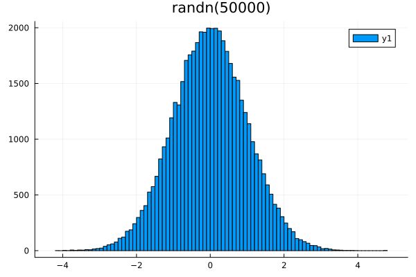
The randn() function generates a normal distribution of numbers with mathematical expectation 0 and the standard deviation 1. (i.e. the range of values will be )
histogram(randn(50000),bims=0.005) # bims - the width of the column into which the point falls
title!("randn(50000)")
The importance of choosing the correct distribution of a random variable
Let's consider such a task:
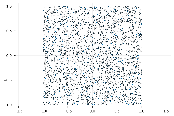
Create a set of points inside a circle of radius R=1 and centered in (0,0), whose Cartesian coordinates are uniformly distributed along the abscissa and ordinate axes. For this
- Create a set of points that fall into a square with a diagonal passing through the vertices
(-1,1), (1,-1) - Select the points that fall within the unit circle.
Step 1.
To solve this step, it is necessary to remember that we want to get evenly distributed values. X in the range of [-1,1]. But rand() - SNRR (i.e. [0,1)).
SNRR possesses by the scaling property:
If a random variable and Then
In our case and
POINTS_NUMBER = 3000
big_square_points = -1 .+ 2. .* rand(POINTS_NUMBER, 2)  # we used the SNR property
In order to avoid using the same keywords each time when plotting graphs, you can add PlotThemes and write the necessary words "by default".
Pkg.add("PlotThemes")
theme(:default, aspect_ratio=1, label = false, markersize=1)
scatter(big_square_points[:,1],big_square_points[:,2])
Step 2
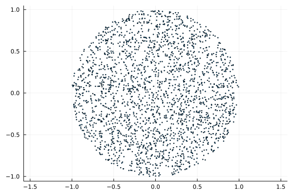
We will go through all the points of our square and add to the array those coordinates that fall within the unit circle.
circle_points_x = Float64[]
circle_points_y = Float64[]
R = 1
for (x, y) in eachrow(big_square_points) # (there are 2 elements in each row of big_square_points: x and y)
if x^2 + y^2 < R^2
push!(circle_points_x, x)
push!(circle_points_y, y)
end
end
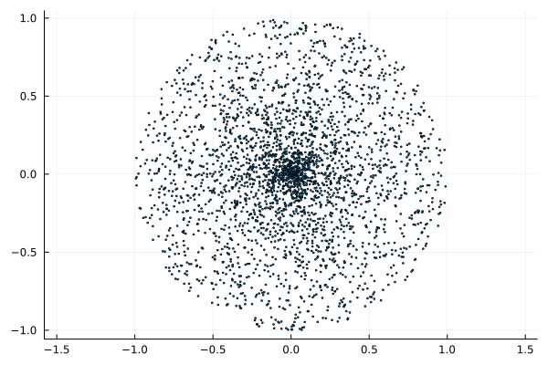
scatter(circle_points_x,circle_points_y)
To solve our problem, a more natural approach would be to use polar coordinates rather than Cartesian coordinates.
Using polar coordinates
Then this task will be reduced to one, not two steps.:
Step 1
Choose and
ρ = rand(POINTS_NUMBER)
α = 2π * rand(POINTS_NUMBER)
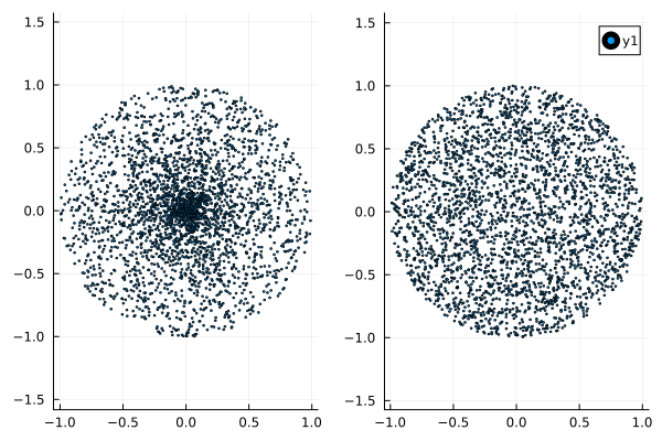
polar_original = scatter(ρ .* cos.(α), ρ .* sin.(α), aspect_ratio=1,markersize=1) # switched back to Cartesian
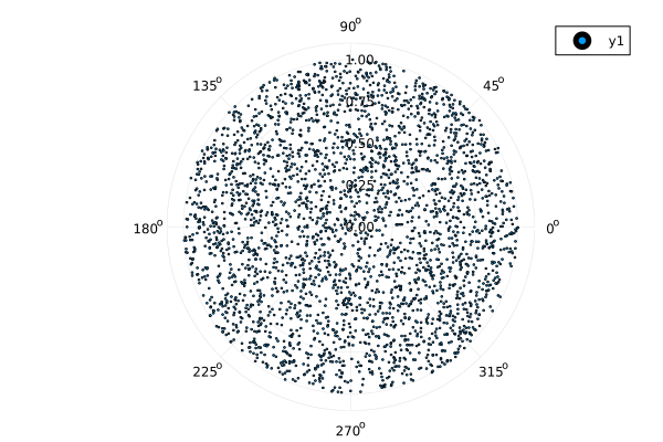
You can also view our results immediately, without switching to Cartesian coordinates. To do this, first disable aspect_ratio=1 and specify proj=:polar - polar mapping.
theme(:default)
scatter(α, ρ , proj=:polar, markersize=1)
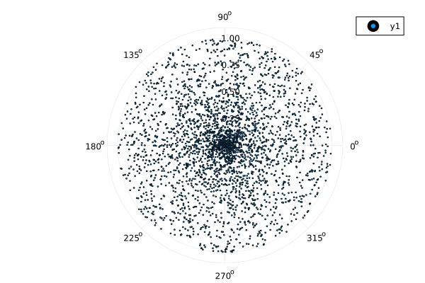
We can see that the density of points near the origin is higher than near the circle.
For clarity, we will cut out an inscribed square from the circle.
To do this, we will use the function zip():
for i in zip(1:5,'a':'e',["🟥","🟩","🟦"])
    println(i)
end
# 4,5 and 'd', 'e' will not be printed, because the color collection ended at step 3
Visualization of point density
small_square_points_x = Float64[]
small_square_points_y = Float64[]

for (x, y) in zip(circle_points_x, circle_points_y)
    if abs(x) ≤ √2 / 2 && abs(y) ≤ √2 / 2
        push!(small_square_points_x, x)
        push!(small_square_points_y, y)
    end
end
small_square_points_ρ = Float64[]
small_square_points_α = Float64[]

for (x, y) in zip(ρ .* cos.(α), ρ .* sin.(α))
    if abs(x) ≤ √2 / 2 && abs(y) ≤ √2 / 2
        push!(small_square_points_ρ, x)
        push!(small_square_points_α, y)
    end
end
To show several graphs on the same canvas at once, you must use layout and specify the structure of their location (in our case, the grid . Using histogram2d we will be able to see which area has a high density of points.
p1 = scatter(   small_square_points_x, small_square_points_y,
                markersize=1, legend = false, aspect_ratio=1)
p2 = scatter(   small_square_points_ρ, small_square_points_α,
                markersize=1, legend = false, aspect_ratio=1)
p3 = histogram2d(small_square_points_x,small_square_points_y,
                 title="density in Cartesian coordinates", aspect_ratio=1)
p4 = histogram2d(small_square_points_ρ,small_square_points_α,
                 title="density in polar coordinates",aspect_ratio=1)

plot(p1,p2,p3,p4,layout=(2,2),size=(950,950))
Function repeat()
Consider the function repeat()
repeat([1:3;],2)
repeat([1:3;],1,2)
repeat([1:3;],2,3)
repeat([1:3;],inner=2)
Comparison of polar and Cartesian coordinates
To understand why the application of polar coordinates and a random uniform distribution over and If they worked in this way, and not, perhaps, in the expected way, consider the following picture.
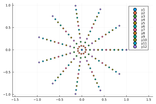
Let's take not a random, but a fixed uniform distribution.:
lngt = 12
a = repeat(range(0, stop=2pi,length=lngt),1,lngt)
r = repeat(range(0, stop=1, length=lngt),1,lngt)'
scatter(r .* cos.(a), r .* sin.(a),aspect_ratio=1, markersize=3)
x = repeat(range(0, stop=1, length=lngt),1,lngt)'
y = repeat(range(0, stop=1,length=lngt),lngt)
scatter(x, y,aspect_ratio=1)
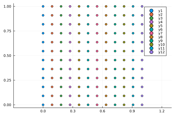
As you can see, the density of the distribution of points in Cartesian coordinates is constant, and in polar coordinates, the density is near the origin.
To solve the problem, we need to use a distribution that is more likely to put a point closer to the end of the radius vector than to the beginning. Let's assume that such a distribution should be linear (the closer to the end, the more likely). It is called triangular.
Triangular distribution
To use the triangular distribution, connect the library Distributions. This library has a large set of different states (in particular, one-dimensional ones). You can familiarize yourself with this set in the documentation.
using Pkg
Pkg.add("Distributions")
using Distributions
Now let's create a set of points with a triangular distribution. To do this, as the first argument of the function rand() We'll pass it on TriangularDist(a,b,c) with parameters a=0,b=1,c=1.
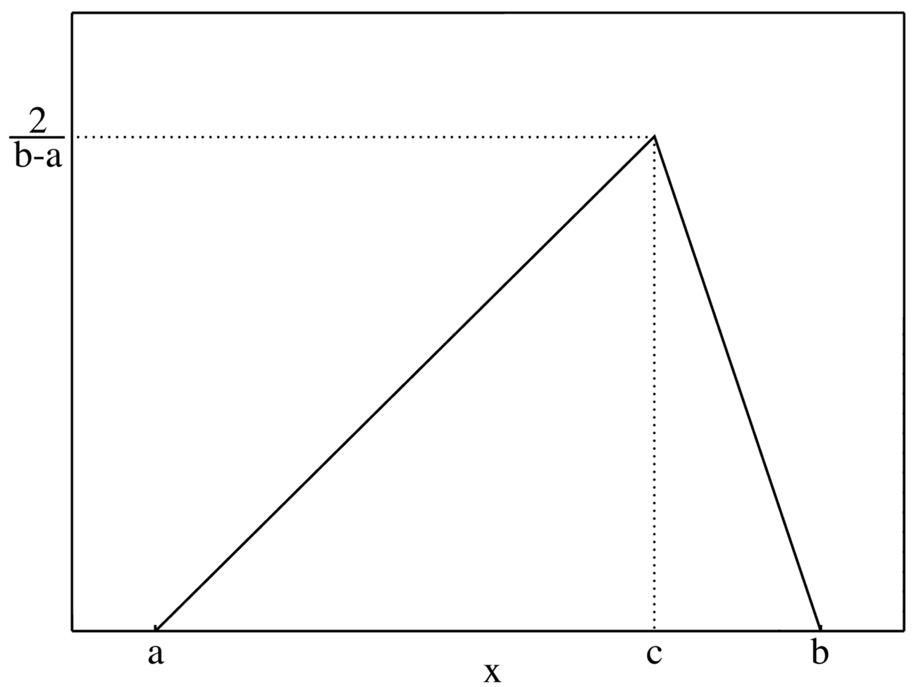
histogram(rand(TriangularDist(0,1,1),POINTS_NUMBER))
After making sure that the triangular distribution works as expected, let's check that its application will solve our problem.:
ρ_triang = rand(TriangularDist(0,1,1), POINTS_NUMBER)
α_triang = rand(Uniform(0,2π), POINTS_NUMBER)    # Uniform(0.2π) - uniform distribution from 0 to 2π
polar_triang = scatter(ρ_triang .* cos.(α_triang), ρ_triang .* sin.(α_triang),aspect_ratio=1, markersize=1)
plot(polar_original, polar_triang,layout=(1,2))
As an interesting fact, we'll show you how to connect the library without Distributions it was possible to solve this problem by adding just two characters. .√ :
ρ_sqrt = .√rand(POINTS_NUMBER)
α_sqrt = 2π * rand(POINTS_NUMBER)
scatter(α_sqrt, ρ_sqrt, proj=:polar, markersize=1)
This is true because:
Using a uniform distribution generator, you can get a triangular distribution generator.:
Conclusion
In this example, it was shown that the Julia language has both convenient built-in functions and specialized packages that allow you to use domain-specific functions while interacting with standard ones.
The methods of generating arrays were also considered (repeat) and iterating over them (zip and eachrow)