Solving the boundary value problem of ballistics
Consider the shot put challenge at the Olympic Games.
- Given:
- flight time
- initial positions and
- end positions and
Determine the initial velocity of the core and the angle of its throw and
Derivation of the ballistics equation
To solve the problem, it is necessary to make up the equations of motion of the thrown object.:
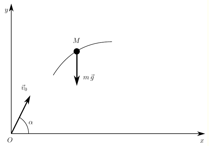
Based on the figure, we will draw up the equations of motion of ballistics.:
By reducing , and passing to the first-order ODE system, we obtain:
Add (Pkg.add) and connect the libraries:
BoundaryValueDiffEqto solve the boundary value problem of differential equationsPlots- to display a graph of solutionsLinearAlgebra: normto find the normPhysicalConstantsIt allows you to use the value of the standard acceleration of free fall
using Pkg
Pkg.add(["BoundaryValueDiffEq","LinearAlgebra","PhysicalConstants"])
using BoundaryValueDiffEq
using Plots
import LinearAlgebra: norm  # We do not use the entire module, but only a specific function.
import PhysicalConstants.CODATA2018: g_n
g_n It is not just a number, but a physical constant (value, dimension, uncertainty of magnitude). To get a "clean" value, you need to use float(g_n). She will return 9.80665 m s^-2. To get only the value, you need to refer to the field val
g_n
const g = float(g_n).val
Now consider прием , which allows you to insert "stubs"
_,b,_,d = [1 2 3 4]
print("b=$b, d=$d")
Let's write down our system of equations
as a function ballistic!(du,u,p,t).
p - system parameters, t - time (but our system is autonomous (stationary), i.e. it clearly does not depend on t).
Don't be afraid to introduce new variables dx, ..., v_y for the sake of improving readability. Most of the time, this does not affect performance.
function ballistic!(du, u, p, t)
    _, _, v_x, v_y = u

    du[1] =  dx  = v_x
    du[2] =  dy  = v_y
    du[3] = dv_x = 0
    du[4] = dv_y = -g
end
Defining the boundary conditions of a problem
Now let's introduce boundary conditions in the initial (a) and the final (b) time points.
These restrictions are introduced in the following form: .
That is, if the condition Then
We will take the task values themselves based on the world record in the shot put.:
- - based on page 13 исследования
- - Olympic record for 2023
- = 0
- (based on the shot_put.mp4 video framing of the record itself)
function bca!(resid_a, u_a, p)
    resid_a[1] = u_a[1]        # x(0) = 0
    resid_a[2] = u_a[2] - 2.1  # y(0) = 2
end

function bcb!(resid_b, u_b, p)
    resid_b[1] = u_b[1] - 23.1  # x(t_f) = 95
    resid_b[2] = u_b[2]       # y(t_f) = 0
end

tspan = (0., 2)
Let's make assumptions about the initial conditions
α = deg2rad(45)
x₀ = 0
y₀ = 2.1
v₀ = 10
v_x_0 = v₀ * cos(α)
v_y_0 = v₀ * sin(α)
u₀ = [x₀, y₀, v_x_0, v_y_0]
Solving a two-point boundary value problem
Let's set a two-point boundary value problem (TwoPointBVProblem).
This problem consists of a system of differential equations, boundary conditions, initial assumptions, and an integration time interval.
The key word bcresid_prototype allows you to set the type of initial assumptions (we can have 4 conditions at a point a and 4 conditions at a point b. But we only specified 2 limits each, since the speeds were not limited at the beginning and at the end.
bvp = TwoPointBVProblem(ballistic!, (bca!, bcb!), u₀, tspan;
        bcresid_prototype=(zeros(2), zeros(2)))
Now it remains to solve the problem by choosing two methods - Shooting, with a solver Verns7(). For more information about algorithms for solving boundary value problems, see документации.
sol = solve(bvp, Shooting(Vern7()), saveat=0.1)
gr()  # We use a static graph display.
plt_record = plot(  sol[1, :], sol[2, :],
                    aspect_ratio=1.0, xlabel="x, m",ylabel="y, m", label = "The trajectory")
scatter!(plt_record, [0,23.1],[2.1, 0],label="boundary conditions")
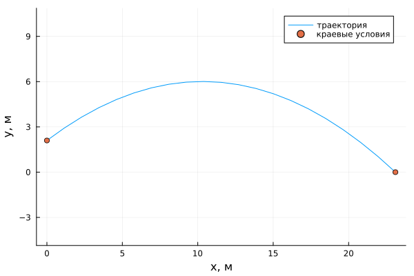
As can be seen from the figure, the solution of the ODE system does indeed satisfy the boundary conditions.
Now we find out the values of the modulus and angle of the velocity vector at the moment of the throw .
norm([3 4]) # √(3²+4²)
norm([sol[1][3],sol[1][4]]) # √(v_x²+v_y²)
x |> f equivalent to f(x)
atan(sol[1][4]/sol[1][3]) |> rad2deg
Thus, the speed of the throw is ≈ 14.5 м/с, and the angle of the throw ≈ 37.16°
Determining the angle of the throw that allows you to reach the target at the lowest initial velocity.
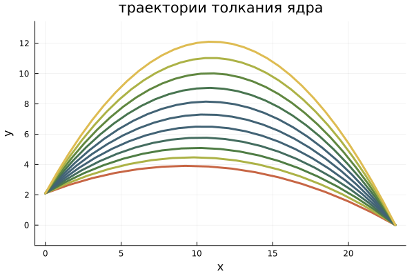
Now let's look at a set of trajectories, and make sure that an angle of 45 ° allows you to reach the target at the lowest initial velocity.
Functions that allow you to change the color of the trajectory, depending on the initial velocity
Before building the trajectories, we define the functions that will allow us to display the color of the line depending on the value of the initial velocity.
Let's write a function map_range, proportionally displaying the number from the segment [a,b] in the segment [A,B].
As parameters, it contains:
- a tuple of two numbers
(a,b)- the initial segment from which it is planned to display - a tuple of two numbers
(A,B)- the segment where
3 is planned to be displayed. - the number of[a,b], which is planned to be displayed in[A,B]
If , then the function throws исключение. In our case, the type of this exception is DomainError, since x leaves the scope of the function definition.
map_range((a, b), (A, B), x) = a < x < b ?
                           A + (x - a) / (b - a) * (B - A) :
                           throw(DomainError(x, "x must be in domain ($a, $b)"))
map_range((14,18),(0,1),15)

# |14---15___16___17___18| |0---0.25___0.5___0.75___1|
# map_range((14,18),(0,1),19) # uncomment it to check how exceptions work.
In order to work with colors and use certain color sets, libraries must be connected. Colors and ColorSchemes
Pkg.add(["Colors","ColorSchemes"])
using Colors
using ColorSchemes
Let's create a set of 20 colors ranging from blue to red.:
COLORS_NUMBER = 20
ndr = ColorScheme(get(ColorSchemes.darkrainbow, range(0.0, 1.0, length=COLORS_NUMBER)))

[ndr[1],ndr[end]]
Let's assume that we will have a set of trajectories, the initial velocities of which will vary from 14 to 17. And we want to find the color corresponding to speed 15, if blue is the lowest speed, red is the highest.
round(Int,3.5)
ndr[round(Int,map_range((14,17),(1,COLORS_NUMBER),15))]

Let's add empty graphs to which we will add new data in each iteration.:
plt_trajectories = plot()
scatter_v_0_α = scatter();
for tspan in map(x -> (0, x), 1.5:0.15:3)
# solving a boundary value problem for a given (t_0,t_f)
bvp = TwoPointBVProblem(ballistic!, (bca!, bcb!), u₀, tspan;
bcresid_prototype=(zeros(2), zeros(2)))
sol = solve(bvp, Shooting(Vern7()), saveat=0.1)
# definition of v_0 and α
v_0 = round(norm([sol[1][3],sol[1][4]]),digits=2) # (round, π, digits=4) = 3.1416
α = atan(sol[1][4]/sol[1][3]) |> rad2deg
# plotting graphs
# # building trajectories
plot!( plt_trajectories, sol[1, :], sol[2, :], aspect_ratio=1.0,
color=ndr[round(Int,map_range((14,17), (1,COLORS_NUMBER),v_0))],
label=nothing, w=3,xlabel="x",ylabel="y", title="the trajectories of the shot put")
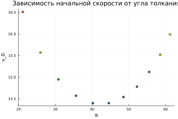
# # to build the dependency v_0(α)
scatter!(scatter_v_0_α,[α],[v_0],label=nothing,
xlabel="α", ylabel="v_0",title="Dependence of the initial velocity on the angle of impact",
color=ndr[round(Int,map_range((14,17), (1,COLORS_NUMBER),v_0))])
end
display(plt_trajectories)
display(scatter_v_0_α)
Conclusions
We can conclude that indeed, in order to achieve the goal (throwing a shot at a certain distance), an angle of 45° provides the minimum initial velocity at which this throw is possible. In other words, an angle of 45° provides the maximum distance that the core can cover if the specified initial velocity is fixed.
As a result of completing the task, the following issues were considered:
- solving a two-point boundary value problem
- the use of physical constants
- creation of functions that throw exceptions when going beyond the boundaries of the function definition area
- custom color change of the trajectories depending on the data corresponding to the trajectory (v_0, in our case)