Implementation of a finite-difference scheme for solving the Laplace equation

In this example, we will solve the following Laplace equation

using a 5-point finite difference solution scheme.

Creating a grid

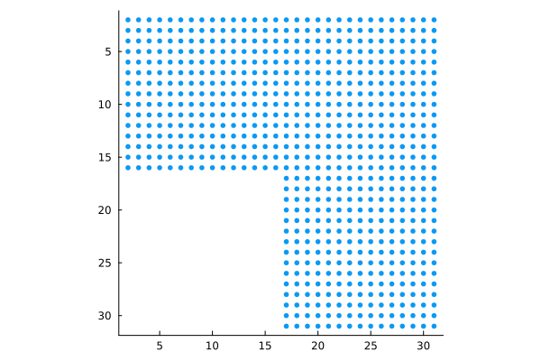
Suppose we are interested in solving a problem on a specific grid defined in the form of an L-shaped group of points on a plane.

Pkg.add(["LinearAlgebra"])

gr()

Plots.GRBackend()

First, we will create a simple matrix of zeros, then fill in the necessary areas with ones, also adding a 1-element "border" to set Dirichlet boundary conditions. Function spy from a set of graphs gr() It is well suited for visualizing areas where the values of matrix elements are nonzero.

10÷2

5

function lshape(N)
    # N = round(Int, N/2) * 2 # make sure that the input parameter is even
    L = zeros(Int, N, N)       # creating an array of Int numbers with a value of 0
    
    # fill in the required area with units
    L[2:N÷2, 2:N-1] .= 1
    L[2:N-1,   N÷2+1:N-1] .= 1
    # ÷ stands for integer division
    # (! julia does not allow indexing vectors using Float numbers)

    # Instead of units, we substitute the numbers of the values in the matrix
    items = findall( !iszero, L )
    L[items] = 1:length(items)

    return L

end

G = lshape( 32 );
spy( G .> 0, markersize=3, markercolor=1 )

If we need to number all these points, how does the function do it? numgrid for the MATLAB platform, use the following code:

g = lshape( 10 ) .> 10

10×10 BitMatrix:
 0  0  0  0  0  0  0  0  0  0
 0  0  0  0  1  1  1  1  1  0
 0  0  0  0  1  1  1  1  1  0
 0  0  0  1  1  1  1  1  1  0
 0  0  0  1  1  1  1  1  1  0
 0  0  0  0  0  1  1  1  1  0
 0  0  0  0  0  1  1  1  1  0
 0  0  0  0  0  1  1  1  1  0
 0  0  0  0  0  1  1  1  1  0
 0  0  0  0  0  0  0  0  0  0

g = lshape( 10 )

10×10 Matrix{Int64}:
 0  0  0   0   0   0   0   0   0  0
 0  1  5   9  13  17  25  33  41  0
 0  2  6  10  14  18  26  34  42  0
 0  3  7  11  15  19  27  35  43  0
 0  4  8  12  16  20  28  36  44  0
 0  0  0   0   0  21  29  37  45  0
 0  0  0   0   0  22  30  38  46  0
 0  0  0   0   0  23  31  39  47  0
 0  0  0   0   0  24  32  40  48  0
 0  0  0   0   0   0   0   0   0  0

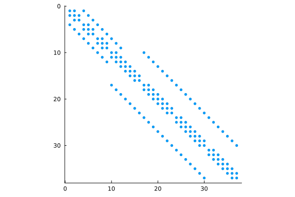
You can see which element numbers of the input matrix should be involved in calculating which results. With a 5-element scheme, elements 1, 2, and 5 (adjacent elements) participate in the calculations of element 1.

The Laplace operator

Now let's load a function that defines the Laplace operator on an arbitrary grid, using a 4-connected domain for calculations.

using SparseArrays, LinearAlgebra
include( "delsq.jl" ); # Creation of the Laplacian

Let's use the function spy to better see the individual markers.

L = lshape(9);
G = delsq(L);
spy( G .!= 0, colorbar=false, markersize=3, markercolor=1 )

Although the standard output for sparse matrices is already quite good at showing areas of different values.

delsq( lshape(9) )

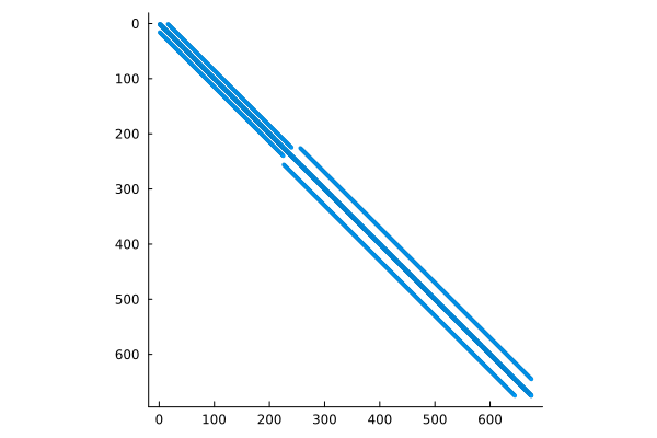
37×37 SparseMatrixCSC{Float64, Int64} with 157 stored entries:
⎡⡻⢎⡢⡀⠀⠀⠀⠀⠀⠀⠀⠀⠀⠀⠀⠀⠀⠀⠀⎤
⎢⠈⠪⡛⣬⡢⡀⠀⠀⠀⠀⠀⠀⠀⠀⠀⠀⠀⠀⠀⎥
⎢⠀⠀⠈⠪⡱⣮⡀⠀⠢⡀⠀⠀⠀⠀⠀⠀⠀⠀⠀⎥
⎢⠀⠀⠀⠀⠀⠈⠻⣦⠀⠈⠢⡀⠀⠀⠀⠀⠀⠀⠀⎥
⎢⠀⠀⠀⠀⠈⠢⡀⠀⠻⣦⡀⠈⠢⡀⠀⠀⠀⠀⠀⎥
⎢⠀⠀⠀⠀⠀⠀⠈⠢⡀⠈⠻⢆⡀⠈⠢⡀⠀⠀⠀⎥
⎢⠀⠀⠀⠀⠀⠀⠀⠀⠈⠢⡀⠈⠻⣦⡀⠈⠢⡀⠀⎥
⎢⠀⠀⠀⠀⠀⠀⠀⠀⠀⠀⠈⠢⡀⠈⠛⣤⡀⠈⠂⎥
⎢⠀⠀⠀⠀⠀⠀⠀⠀⠀⠀⠀⠀⠈⠢⡀⠈⠻⣦⡀⎥
⎣⠀⠀⠀⠀⠀⠀⠀⠀⠀⠀⠀⠀⠀⠀⠈⠀⠀⠈⠁⎦

And for a 32*32 matrix (we will output a part of this matrix):

G = lshape( 32 );
D = delsq( G );
spy( D .!= 0, colorbar=false, markersize=2, markershpe=:square, markercolor=1 )

How many points are there in total in this function (roughly speaking, how many calculations it sets):

N = sum( G[:] .> 0 )

675

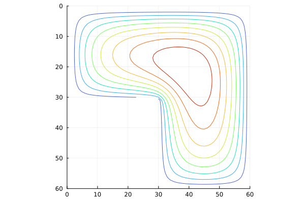
Solving the PDE with a boundary condition

Now we are ready to solve the above differential equation with the Dirichlet boundary condition (1 if the point is inside the domain, 0 if it is on the boundary). Julia easily allows you to solve linear systems of equations with coefficients in the form of sparse matrices (using the [UMFPack] library (http://faculty.cse.tamu.edu/davis/suitesparse.html ) – the same as MATLAB).

N = 60                   # Let's define the right-hand side of the equation
L = lshape(N)
A = -delsq(L)
b = ones( size(A,1) ) / N^2

u = A \ b;          # Solving a system of linear equations

Let's draw a contour graph of this solution.:

U = zeros( size(L) )
U[findall(!iszero, L)] = u

contour( U, levels=8, xlimits=(0,N), ylimits=(0,N), 
         yflip=true, c=cgrad(:turbo, rev=true),
         cbar=false, aspect_ratio=:equal )

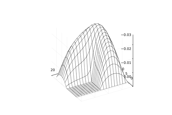
Now let's output the solution as a three-dimensional grid.:

wireframe( U[1:3:end,1:3:end],
           zflip=true, camera=(240,30),
           fmt=:png, aspect_ratio=:equal )

Conclusion

We solved a simple equation on an L-shaped calculation grid, which was set using a function we wrote. In addition, since we used sparse matrices, our task should be solved faster and take up less memory than when using dense (conventional) matrices, thus, theoretically, we get the opportunity to solve many times larger tasks.