Modelling of an electric oscillating circuit¶

Introduction¶

In this example, the modelling of an electrical oscillating circuit will be discussed and the use of the Engee Function block of the Engee modelling environment will be discussed.

Task:

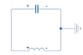
An electrical circuit consisting of an ideal capacitor of capacitance C = 1 F, an ideal inductor of inductance L = 1 Gn and an earth connection is given. Suppose that at the initial moment of time the capacitor is charged to 1 V and there is no current in the circuit.

Construct the Cauchy problem for the system of ordinary differential equations corresponding to the circuit diagram and write a programme to solve it by any numerical method on the interval t ∈ [0; 100]. Give the graphs of change of current and voltage of the capacitor. Justify the correctness of the obtained solution both from the point of view of physics of the process and from the point of view of mathematics.

Calculation algorithm¶

Solution: The electrical circuit given in the problem corresponds to the differential equation of undamped oscillations in an oscillating circuit:

$$U+L \frac{dl}{dt}=0,$$

Where $U=\frac{q}{c}$ is the voltage across the capacitor, $i=-\frac{dq}{dt}$ is the current, and $\frac{di}{dt}=-\frac{d^2q}{dt^2}$ is the change in current.

Then the equation above takes the form:

$$L\frac{d^2q}{dt^2}-\frac{q}{c}=0$$

In order to lower the order of the derivative, variable substitution was applied: $q=y_1, \frac{dq}{dt}=y_2$. As a result, a system of equations is obtained:

$$\begin{cases}\frac{dy_1}{dt}=y_2 \\\frac{dy_2}{dt}=\frac{y_1}{LC}\end{cases}$$

To the obtained system we apply the formula of Euler's method and obtain:

$$Y1(i)=Y1(i-1) + h*Y2(i),$$ $$Y2(i)=Y2(i-1) - h * (Y1(i-1)/(L*C))$$

Implementation of the calculation algorithm in the Julia language:

Pkg.add(["CSV"])

using Plots #импорт графической библиотеки
n = 1000; #количество шагов расчёта
U = fill(0.0,n); #определение массивов
Y1 = fill(0.0,n);
Y2 = fill(0.0,n);
t = fill(0.0,n);
U[1] = 1.0; #напряжение источника в начальный момент времени, на первом шаге расчёта
C = 1.0; #ёмкость конденсатора
L = 1.0; #индуктивность
Y1[1] = 0.0; #сила тока
Y2[1] = U[1]/L; #скорость изменения силы тока
h = 0.1; #величина шага расчёта
t[1] = 0.0; #время на первом шаге расчёта
for i=2:n #начало цикла
    Y2[i] = Y2[i-1] - h * (Y1[i-1] / (L * C));
    Y1[i] = Y1[i-1] + h * Y2[i];
    U[i] = U[i-1] - h * (Y1[i] / C);#изменение напряжения, полученное из формулы U=q/C, где q - заряд конденсатора, а С - его ёмкость
    t[i] = t[i-1] + h;
end
I = Y1;

Visualisation of calculated parameters¶

Calculation results obtained during the implementation of the model:

plotlyjs()
plot(t, I, xlabel="t", ylabel="", title="Напряжение U и ток I", linecolor =:blue, bg_inside =:white, line =:solid, label = "I")
plot!(t, U, xlabel="t", ylabel="", title="Напряжение U и ток I", linecolor =:red, bg_inside =:white, line =:dashdot, label = "U")

Realisation of the model run in Engee using software control¶

Loading the model:

modelName = "LC_model";
LC_model = modelName in [m.name for m in engee.get_all_models()] ? engee.open( modelName ) : engee.load( "$(@__DIR__)/$(modelName).engee");

Running a loaded model:

data = engee.run( modelName )

Dict{String, DataFrames.DataFrame} with 2 entries:
  "current" => 1001×2 DataFrame…
  "voltage" => 1001×2 DataFrame…

Load and visualise the data generated by the simulation¶

Reading csv files with voltage and current variation data, with subsequent conversion to dataframe and matrix.

using CSV, DataFrames

voltage = data["voltage"];
current = data["current"];

Connection of a library for plotting:

using Plots

Plotting a graph describing a change in voltage.

plot(voltage.time, voltage.value, xlabel="Время, с", ylabel="Амплитуда", title="Напряжение U и ток I", linecolor =:red, bg_inside =:white, line =:dashdot, label = "U")
plot!(current.time, current.value, xlabel="Время, с", linecolor =:blue, bg_inside =:white, line =:solid, label = "I")

Conclusion¶

In this example we have demonstrated the calculation of LC loop oscillations using a script and in a visual modelling environment using the Engee Function block.

As can be seen from the graphs - the oscillations are undamped, since there are only ideal elements in the circuit, not taking into account energy dissipation. The frequency of oscillations obtained in the simulation corresponds to the one calculated by the formula $f=\frac{1}{2\pi\sqrt{LC}}$ and is 0.1591 Hz, the period of oscillations is 6.28 s.